Chapter 9 Deep Learning — MLP Neural Networks Explained

This is an Open Access web version of the book Practical Machine Learning with R published by Chapman and Hall/CRC. The content from this website or any part of it may not be copied or reproduced. All copyrights are reserved.

If you find an error, have an idea for improvement, or have a question, please visit the forum for the book. You find additional resources for the book on its companion website, and you can ask the experimental AI assistant about topics covered in the book.

If you enjoy reading the online version of Practical Machine Learning with R, please consider ordering a paper, PDF, or Kindle version to support the development of the book and help me maintain this free online version.

Deep Learning is an Artificial Intelligence (AI) methodology. It performs tasks that we all believed just a few years ago, could only be performed by humans.

Deep Learning models are used in many different applications. For example, researchers use Deep Learning to analyze medical images to improve cancer diagnosis (image recognition); Amazon’s Alexa uses Deep Learning to understand human languages (Natural Language Processing (NLP)); and you can use Conversational Generative Pre-training Transformers (short: chatbots) like ChatGPT from OpenAI or Bard from Google to compose written text or just have a chat. These technologies are all based on Deep Learning.

Deep Learning uses Neural Networks as integral part. There would be no Deep Learning without Neural Networks. The term Neural Networks originated from early attempts of researchers (see for example McCulloch and Pitts (1943)) to create machine learning models that resemble the human brain.

The human brain processes information as electric currents through neurons, and then passes it on to other neurons connected by dendrites in a complex network with endless layers of neurons. Similarly, a Neural Network contains layers of interconnected nodes — like neurons in the human brain. Each of these nodes, or artificial neurons, performs a mathematical operation on the data it receives, and then passes the results on to other neurons in the network.

Neural Networks research today focuses on improving predictive quality rather than attempting to resemble the human brain. Consequently, in what follows, we will not discuss how little or how much a Neural Network is similar to a human brain. For a brief discussion of this topic, see Haykin (1999), Section 1.2 and Lange (2003), Chapter 2.

The word “deep” in Deep Learning refers to the number of layers in the Neural Network structure. In general, Deep Learning algorithms are extremely complex with many layers and a very high number of parameters to estimate (sometimes billions or trillions of parameters!).⁵⁹ Here are some examples of deep Neural Networks:

• Convolutional Neural Networks (CNN): for image recognition and classification.

• Recurrent Neural Networks (RNN): for sequence processing.

• Long short-term memory (LSTM): a more advanced type of RNN for tasks that require sequence processing, such as speech recognition and sentiment analysis.

• Generative Adversarial Networks (GANs): for semantic image editing, style transfer, image synthesis.

• Generative AI: a field that is still developing. Applications so far reach from generating reports, papers and art; all the way to simulation of scientific experiments. The end of future applications is not in sight.

Due to the complexity and the demanding computational resources, Deep Neural Networks are beyond the scope of this chapter. Instead, we will explain the basic underlying concepts of Deep Learning using a simpler Neural Network type called Multi-Layer Perceptron (MLP).

MLP Neural Networks were among the first Neural Networks to be developed. The principles of MLP Neural Networks can also be applied to more complex and sophisticated Neural Networks. After reading this chapter you will have a good idea about the basic functionality of Deep Neural Networks.

MLP Neural Networks consist of one or more layers, each layer contains at least one neuron. The layers in MLP Neural Networks are fully connected, meaning that each neuron in one layer can pass information to each neuron in the following layer. Figure 9.1 in Section 9.4.1 shows a basic example of a fully connected MLP Neural Network with an input layer (2 neurons), a hidden layer⁶⁰ (2 neurons), and an output layer (1 neuron).

Neural Networks can be used for classification and regression tasks. Here, we will focus on regression tasks. Throughout this chapter, we will use the diamonds dataset⁶¹ to predict diamond prices based on a diamond’s physical properties. We will introduce the diamonds dataset in more detail in Section 9.3.

In what follows, MLP Neural Networks are covered in four parts:

In Section 9.4,

we introduce the idea behind Neural Networks in an intuitive way. We show the structure of a simplified Neural Network, demonstrating how a Neural Network predicts, and we describe the basic principle (Back Propagation/Steepest Gradient Descent) used by the Optimizer to find the best \(\beta\) parameters for a Neural Network.

In Section 9.5

we use the nnet R package (Venables and Ripley (2002)) together with tidymodels and the diamonds dataset to predict diamond prices using a MLP Neural Networks model. The nnet package has been around for a long time, and more advanced packages have been developed. However, we use nnet in Section 9.4 because it supports Sigmoid activation functions, which allows us to introduce basic ideas of Neural Network algorithms in a straightforward way.

In Section 9.6

we compare the R nnet package and PyTorch, another open source machine learning library using Neural Networks. The latter is implemented through the brulee package (Kuhn and Falbel (2022)) into R. PyTorch is a machine learning framework initially developed by Facebook (now Meta AI). It provides MLP Neural Network functionality that supports more advanced activation functions (e.g., the Rectified Linear Unit (ReLU) activation function) and more tuning parameters to optimize predictive performance.

In the interactive Section 9.7

you will use PyTorch to estimate diamond prices in a real-world setting. We will provide a template that allows you to try various hyper-parameter settings for tuning the Neural Network model.

9.1 Learning Outcomes

This section outlines what you can expect to learn in this chapter. In addition, the corresponding section number is included for each learning outcome to help you to navigate the content, especially when you return to the chapter for review.

In this chapter, you will learn:

• How to work with a graphical representation of a Neural Network (see Section 9.4.1).

• How to transform the graphical representation into a Neural Network prediction function (see Section 9.4.2).

• How to use an Optimizer in a Neural Network to change the network’s parameters to step-wise improve the approximation quality (the underlying method is called Steepest Gradient Decent or Back Propagation Algorithm; see Section 9.4.4)

• Why Neural Networks have outstanding approximation qualities that allow them to approximate any continuous function with any degree of accuracy (see Section 9.5).

• How and why the outstanding approximation quality of Neural Networks makes them prone to overfitting (see Section 9.5).

• How to work with the R nnet package and with PyTorch to design and run a Neural Network (see Section 9.5 and Section 9.7).

• Why a Neural Network with ReLU (Rectified Linear Unit) activation functions has the same outstanding approximation properties as a Neural Network with classic Sigmoid activation functions (see Section 9.6).

• Why ReLU functions mitigate the possible inability of the Optimizer to change the values for the \(\beta\) parameters (Vanishing Gradient problem; see Section 9.6).

• How to use PyTorch in an interactive project to estimate the prices of more than \(50{,}000\) diamonds based on four common predictors used in the appraisal industry (Carat, Clarity, Cut, and Color; see Section 9.7).

9.2 R Packages Required for the Chapter

This section lists the R packages that you need when you load and execute code in the interactive sections in RStudio. Please install the following packages using Tools -> Install Packages \(\dots\) from the RStudio menu bar (you can find more information about installing and loading packages in Section 3.4):

• The rio package (Chan et al. (2021)) to enable the loading of various data formats with one import() command. Files can be loaded from the user’s hard drive or the Internet.

• The janitor package (Firke (2023)) to rename variable names to UpperCamel and to substitute spaces and special characters in variable names.

• The tidymodels package (Kuhn and Wickham (2020)) to streamline data engineering and machine learning tasks.

• The kableExtra (Zhu (2021)) package to support the rendering of tables.

• The learnr package (Aden-Buie, Schloerke, and Allaire (2022)), which is needed together with the shiny package (Chang et al. (2022)) for the interactive exercises in this book.

• The shiny package (Chang et al. (2022)), which is needed together with the learnr package (Aden-Buie, Schloerke, and Allaire (2022)) for the interactive exercises in this book.

• The nnet package (Venables and Ripley (2002)) to create and optimize basic MLP Neural Networks.

• The brulee package (Kuhn and Falbel (2022)) to create and optimize MLP Neural Networks based on the Python library PyTorch. Regarding the brulee package, it is important to mention that the PyTorch software needs to be installed after the package is installed. Installing the PyTorch software is straightforward: When the package is used for the first time (i.e., with library(brulee)) a popup window asks to download and install the required software. After confirming with “Yes”, the software will be installed.

9.3 Data

For training and testing, we use the well-known diamonds dataset. The diamonds dataset contains information on \(53,940\) diamonds and is included in the R package ggplot2 (Wickham (2016)). You can learn more about the diamonds dataset by typing "? diamonds" into the R Console. Since ggplot2 is automatically loaded with the tidymodels package, the command library(ggplot2) is not required.

In the code block below, we first load the tidymodels and janitor libraries. Then we convert the column names in the diamonds data frame to UpperCamel, select the variables \(Price\), \(Carat\), \(Clarity\), \(Cut\), and \(Color\) for the analysis, and save the result into the data frame DataDiamonds. Afterwards, we use the str() command to take a look at the structure of the data frame:

library(tidymodels); library(janitor)
DataDiamonds= diamonds |> 
              clean_names("upper_camel") |> 
              select(Price, Carat, Clarity, Cut, Color)
str(DataDiamonds)

## tibble [53,940 × 5] (S3: tbl_df/tbl/data.frame)
##  $ Price  : int [1:53940] 326 326 327 334 335 336 336 337 337 338 ...
##  $ Carat  : num [1:53940] 0.23 0.21 0.23 0.29 0.31 0.24 0.24 0.26 0.22
##  $ Clarity: Ord.factor w/ 8 levels "I1"<"SI2"<"SI1"<..: 2 3 5 4 2 6 7 
##  $ Cut    : Ord.factor w/ 5 levels "Fair"<"Good"<..: 5 4 2 4 2 3 3 3 1
##  $ Color  : Ord.factor w/ 7 levels "D"<"E"<"F"<"G"<..: 2 2 2 6 7 7 6 5

The output of the str() command shows that the data frame DataDiamonds contains 53,940 observations and five different variables (columns) that describe various properties of the diamonds together with their prices (in U.S.-$).

The variables \(Carat\), \(Clarity\), \(Cut\), and \(Color\) chosen as predictors are also known as the four Cs of diamond appraisal:⁶²

1. Carat: A measurement unit used to describe a diamond’s weight. It is measured in metric grams (1 \(carat\) equal to 0.2 \(g\)) and is the most visually apparent factor when comparing diamonds.

2. Clarity: A measurement for the visibility of natural microscopic inclusions and imperfections within a diamond. Diamonds with little to no inclusions are considered particularly rare and highly valued. The clarity of the diamond is rated in eight categories measuring how clear the diamond is (I1 (worst), SI2, SI1, VS2, VS1, VVS2, VVS1, IF (best)).⁶³

3. Cut: Refers to a diamond’s facets, symmetry, and reflective qualities. The cut of a diamond is directly related to its overall sparkle and beauty. The cut of a diamond is rated in five categories as Fair, Good, Very Good, Ideal, and Super Ideal.

4. Color: Refers to the natural color or lack of color visible within a diamond. The closer a diamond is to “colorless”, the more expensive the diamond is. Color is rated in seven categories from D (best) to J (worst).

From the str() command output above, you can see that \(Clarity\), \(Cut\), and \(Color\) are stored as R factor-data-type with \(8\), \(5\), and \(7\) factor-levels, respectively. Since we need numerical values for the analysis, we use the as.integer() command in the code block below to extract the factor-levels as integer values:

DataDiamonds=DataDiamonds |> 
             mutate(Clarity=as.integer(Clarity)) |> 
             mutate(Cut=as.integer(Cut)) |> 
             mutate(Color=as.integer(Color))
head(DataDiamonds)

## # A tibble: 6 × 5
##   Price Carat Clarity   Cut Color
##   <int> <dbl>   <int> <int> <int>
## 1   326  0.23       2     5     2
## 2   326  0.21       3     4     2
## 3   327  0.23       5     2     2
## 4   334  0.29       4     4     6
## 5   335  0.31       2     2     7
## 6   336  0.24       6     3     7

9.4 The Idea Behind Neural Network Models

This section introduces some of the principle ideas behind Neural Networks. We start in Section 9.4.1 with a graphical representation of a simplified Neural Network that predicts the \(Price\) of a diamond based on two predictor variables (\(Carat\) and \(Clarity\)). In Section 9.4.2, we will show how the graphical representation of a Neural Network can be transformed into the prediction equation of the Neural Network. In Section 9.4.3 we use a numerical example to show how the Neural Network can predict the price of a given diamond based on its \(carat\) and \(clarity\) when the values for the \(\beta\) values are determined. Finally, in Section 9.4.4, we try to shed some light on how the Optimizer in a Neural Network can find the \(\beta\) parameters that lead to the best prediction quality (minimizing the \(MSE\) for the training data).

9.4.1 Graphical Representation of a Neural Network Explained

Let us start with a graphical approach by demonstrating how a Neural Network can predict continuous outcome variables such as the \(Price\) of a diamond based on two predictor variables \((Carat\) and \(Clarity)\).

Figure 9.1 demonstrates the process. The figure shows a Neural Network with an input layer at the left of the network consisting of two input neurons (\(I1\) and \(I2\)), a hidden layer in the middle of the network composed of two hidden neurons (\(H1\) and \(H2\)), and an output layer at the right of the network with one output neuron that will later contain the diamond’s predicted price (\(O1\)).

The three layers (input, hidden, and output) are fully connected with the red and black lines, meaning that each neuron of a previous layer is connected with each neuron of the following layer. Considering that perceptron is a different term for neuron, you can see where the name Multi Layer (input, hidden, output) Perceptron comes from. The MLP in Figure 9.1 has only one hidden layer, but more complex MLP networks can have multiple hidden layers with many neurons inside each layer.

FIGURE 9.1: Graphical Representation of a Neural Network

A Neural Network processes observations one by one and creates a prediction at the output neuron (\(O1\)) for each observation. We will use Figure 9.1 to show how a Neural Network can generate a prediction from the values of the predictor variables of a given observation \(i\). For now, we assume that values for the parameters (the \(\beta s\)) are provided and known:

Step 1:

At the beginning of the prediction process, the values for the predictor variables of observation \(i\) are loaded into the input neurons (\(I1\) and \(I2\)). For example, for a diamond with \(0.3\) carats \((Carat_i=0.3)\) and clarity rating of SI1 \((Clarity_i=3)\), the input neuron \(I1\) contains a value of \(0.3\), and the input neuron \(I2\) contains a value of \(3\).

Step 2:

The values of the input neurons are transmitted to each of the hidden neurons (\(H1\) and \(H2\)), but before they arrive, their values are weighted (multiplied) with the parameters \(\beta_2\), \(\beta_3\), \(\beta_5\), and \(\beta_6\), respectively. This way, the original value from the input neurons are amplified or weakened, depending on whether the absolute values for the \(\beta s\) are greater or smaller than one. Negative \(\beta\) parameter values reverse the signs of the predictor variable values.

In addition to the weighted input values (\(Carat_i \cdot\beta_2\), \(Clarity_i \cdot\beta_3\), \(Carat_i \cdot\beta_5\), and \(Clarity_i \cdot\beta_6\)) that arrive at the hidden neurons \(H1\) and \(H2\), the bias neuron \(B1\) sends a value that is equal to \(\beta_1\) to hidden neuron \(H1\) and a value of \(\beta_4\) to hidden neuron \(H2\). Because these values are independent of the values for the predictor variables (\(B1\) and \(B2\) always contain a value of one), the neurons \(B1\) and \(B2\) are called bias neurons.

Step 3:

As you can see in Figure 9.1 at the green \(\Large\oplus\) signs in front of the hidden neurons \(H1\) and \(H2\), three different weighted values arrive at each hidden neuron before they are further processed. For each hidden neuron, the three related values are aggregated to single values called the effective inputs of the hidden neurons by simply adding them up. This is symbolized by the green \(\Large\oplus\) signs in front of \(H1\) and \(H2\) in Figure 9.1. The effective inputs \((I_{1,i}^{eff}\) and \(I_{2,i}^{eff})\) for the hidden neuron \(H1\) and \(H2\) are:

\[I_{1,i}^{eff}=\beta_1+\beta_2 Carat_i +\beta_3 Carity_i\] and \[I_{2,i}^{eff}=\beta_4+\beta_5 Carat_i + \beta_6 Carity_i\]

Step 4:

These two effective inputs — one for each of the hidden neurons — are now plugged into non-linear functions (called activation functions) inside hidden neuron \(H1\) and \(H2\). The two results are called the activities (\(A^{ct}_{1,i}\) and \(A^{ct}_{2,i}\)) of the neurons \(H1\) and \(H2\). We will talk more about activation functions in a minute.

Steps 5:

The activities of the hidden neurons \(A^{ct}_{1,i}\) and \(A^{ct}_{2,i}\) are transmitted to the output neuron (\(O1\)), but before they arrive, their values are weighted with \(\beta_8\) and \(\beta_9\), respectively.

Steps 6:

Three values arrive at the green \(\Large\oplus\) sign in front of the output neuron (\(O1\)): the two weighted activities from the hidden neurons (\(\beta_8 A^{ct}_{1,i}\) and \(\beta_9 A^{ct}_{2,i}\)) and the value from the bias neuron \(B2\), which equals \(\beta_7\). These three values are aggregated (added up) to a single value, which is the value of the output neuron \(O1\) and, at the same time, the predicted price for the related diamond.

In more complex networks, the output neuron \(O1\) may also contain an activation function, but here what goes into the output neuron comes out without any transformation \((O1=I^{eff}_{O1})\).

The steps above, in connection with Figure 9.1 provide a basic idea about how a Neural Network processes values from predictor variables to generate a prediction for an outcome variable. If the Neural Network contains more input and hidden neurons, or more layers, the process is more complex, but the underlying idea is the same.

However, two questions have not been answered so far:

Question 1:

We assumed that the values for the \(\beta\) parameters are known. But how are they determined?

Answer:

The answer to this question is simple for the initial values of the \(\beta s\): The parameters are determined randomly (usually with \(-1<\beta_j<1)\). This makes it possible to generate initial predictions for all observations in the training dataset. The resulting initial predictions are usually not very good. They need improvement by updating the \(\beta\) parameters in an iterative process. This updating process — called training the Neural Network — is a little more complex. We will discuss the underlying basics in Section 9.4.4 after we cover a numerical example for a prediction in Section 9.4.3.

Question 2:

How are the activation functions inside the hidden neurons \(H1\) and \(H2\) transforming the effective input values \((I^{eff}_{1,i}\) and \(I^{eff}_{2,i})\) into the activities of the hidden neurons \((A^{ct}_{1,i}\) and \(A^{ct}_{2,i})\)?

Answer:

This is a bit more tricky: Various activation functions can be used inside a hidden neuron to transform the effective inputs \(I_{j,i}^{eff}\) into a neurons’ activity \(A^{ct}_{j,i}\) (\(j\) stands for the hidden neuron number and \(i\) for the observation number). Here, we use the Logistic function — the same function we used for Logistic Regression in Chapter 8. We plug the effective inputs \(I_{1,i}^{eff}\) and \(I_{2,i}^{eff}\) into the Logistic function and calculate the activities \(A^{ct}_{1,i}\) and \(A^{ct}_{2,i}\) for the hidden neurons \(H1\) and \(H2\):

\[\begin{eqnarray} A^{ct}_{1,i}&=&\frac{1}{1+e^{-I_{1,i}^{eff}}} \tag{9.1} \\ A^{ct}_{2,i}&=&\frac{1}{1+e^{-I_{2,i}^{eff}}} \tag{9.2} \end{eqnarray}\]

9.4.2 Transforming the Graphic Approach Into a Prediction Equation

Figure 9.1 shows the graphical structure of a Neural Network, but for using a computer to make predictions, the graph needs to be transformed into a prediction equation, which is the goal of this section.

Figure 9.1 and Step 3 above show how the effective inputs for the two hidden neurons are calculated from the weighted predictor variables and the bias neurons. For an observation \(i\), this can be expressed in the following two equations determining \(I_{1,i}^{eff}\) and \(I_{2,i}^{eff}\):

\[\begin{eqnarray} I_{1,i}^{eff}=\beta_1+\beta_2 Carat_i +\beta_3 Clarity_i \tag{9.3}\\ I_{2,i}^{eff}=\beta_4+\beta_5 Carat_i +\beta_6 Clarity_i \tag{9.4} \end{eqnarray}\]

We can substitute \(I_{1,i}^{eff}\) and \(I_{2,i}^{eff}\) according to Equations (9.3) and (9.4) into the activation functions (9.1), and (9.2) and we get the activities for the hidden neurons:

\[\begin{eqnarray} A^{ct}_{1,i}&=&\frac{1}{1+e^{-(\require{color}\colorbox{sandyellowcl}{$\beta_1 +\beta_2 Carat_i+\beta_3 Clarity_i$})}} \tag{9.5}\\ A^{ct}_{2,i}&=&\frac{1}{1+e^{-(\require{color}\colorbox{sandyellowcl}{$\beta_4 +\beta_5 Carat_i+\beta_6 Clarity_i$})}} \tag{9.6} \end{eqnarray}\]

Note, the effective inputs (\(I_{1,i}^{eff}\) and \(I_{2,i}^{eff}\)) for the two hidden neurons are highlighted to make the equations easier to read.

Equations (9.5) and (9.6) show that we can calculate the activities for the hidden neurons \(H1\) and \(H2\) entirely based on the predictor values of an observation if we know the numerical values for the \(\beta s\) (and we do!).

After transforming the activities (\(A^{ct}_{1,i}\) and \(A^{ct}_{2,i}\)) of the two hidden neurons into formulas, we are only two steps away from predicting the price of a diamond. As shown before in Steps 5 and 6, the predicted price can be calculated from the activities of the hidden neurons and the bias neuron as follows:

\[\begin{equation} \widehat {Price}_i =\beta_7 + \beta_8 A^{ct}_{1,i} + \beta_9 A^{ct}_{2,i} \tag{9.7} \end{equation}\]

If we now substitute \(A^{ct}_{1,i}\) and \(A^{ct}_{2,i}\) according to Equations (9.5) and (9.6), we get the Neural Network’s prediction function:

\[\begin{eqnarray} \widehat {Price}_i&=&\beta_7+ \overbrace{ \frac{1}{1+e^{-(\require{color}\colorbox{sandyellowcl}{$\beta_1 +\beta_2 Carat_i+\beta_3 Clarity_i$})}} }^{\mbox{Activity of Hidden Neuron 1}}\cdot \beta_8 \nonumber \\ \nonumber \\ &+& \overbrace{ \frac{1}{1+e^{-(\require{color}\colorbox{sandyellowcl}{$\beta_4 +\beta_5 Carat_i+\beta_6 Clarity_i$})}} }^{\mbox{Activity of Hidden Neuron 2}}\cdot\beta_9 \tag{9.8} \end{eqnarray}\]

Again, for readability, the effective inputs (\(I_{1,i}^{eff}\) and \(I_{2,i}^{eff}\)) for the two hidden neurons are highlighted.

Deriving the prediction function in Equation (9.8) was a little tedious. You might want to go back to Steps 1 – 6 and read again carefully. It is worth the effort because the prediction equation in (9.8) indicates how a Neural Network can predict based on the predictor values when the \(\beta\) parameters are known. If you understand this concept, you will realize that the predictive quality of the Neural Network only depends on the right choice of the parameters (the \(\beta s\)).

The takeaways so far are:

1. The Neural Network from Figure 9.1 can be transformed into a prediction equation (see Equation (9.8)).

2. The predicted price for a diamond following Equation (9.8) depends only on the predictor values (\(Carat\) and \(Clarity\)) and the values for the \(\beta\) parameters.

3. Since we know the values for the \(\beta s\), either from randomly choosing them or as part of the optimization process, we can predict the price for any diamond based on \(Carat\) and \(Clarity\).

4. The initial prediction with a random parameter choice is likely not good, but we can gradually improve the prediction by adjusting the \(\beta\) parameters iteratively. How this can be done will be explained in Section 9.4.4.

If not all details are clear to you at this point, do not worry. We will follow up with a numerical example in the next section.

9.4.3 Numerical Example: Predicting Prices for Diamonds with a Neural Network

In this section, we will choose an individual diamond (see Table 9.1) and predict its price based on the Neural Network displayed in Figure 9.2 and also based on the prediction Equation (9.8).

TABLE 9.1: Sample Diamond from DataDiamonds

Price	Carat	Clarity
506	0.3	3

Table 9.1 shows that the diamond has \(0.3\) carats \((Carat_i=0.3)\) and a clarity of 3 \((Clarity_i=3)\). All other predictors are omitted for now. We assume for the initial prediction that the values of the \(\beta\) parameters are already randomly determined as:

\[\beta_1 = 0.1, \beta_2=-0.9 ,\beta_3=0.5 ,\beta_4 = -0.1, \beta_5 = 0.8, \beta_6 =0.6 ,\] \[\beta_7 =0.1 ,\beta_8 = 0.8,\beta_9 = 0.9\]

The prediction process is displayed in Figure 9.2. The color of the connectors between the neurons shows if the related parameter is positive (black) or negative (red). The connector’s thickness reflects whether the parameter — in absolute terms — is big or small. As an exercise, compare the connectors in Figure 9.2 with the randomly chosen \(\beta\) values.

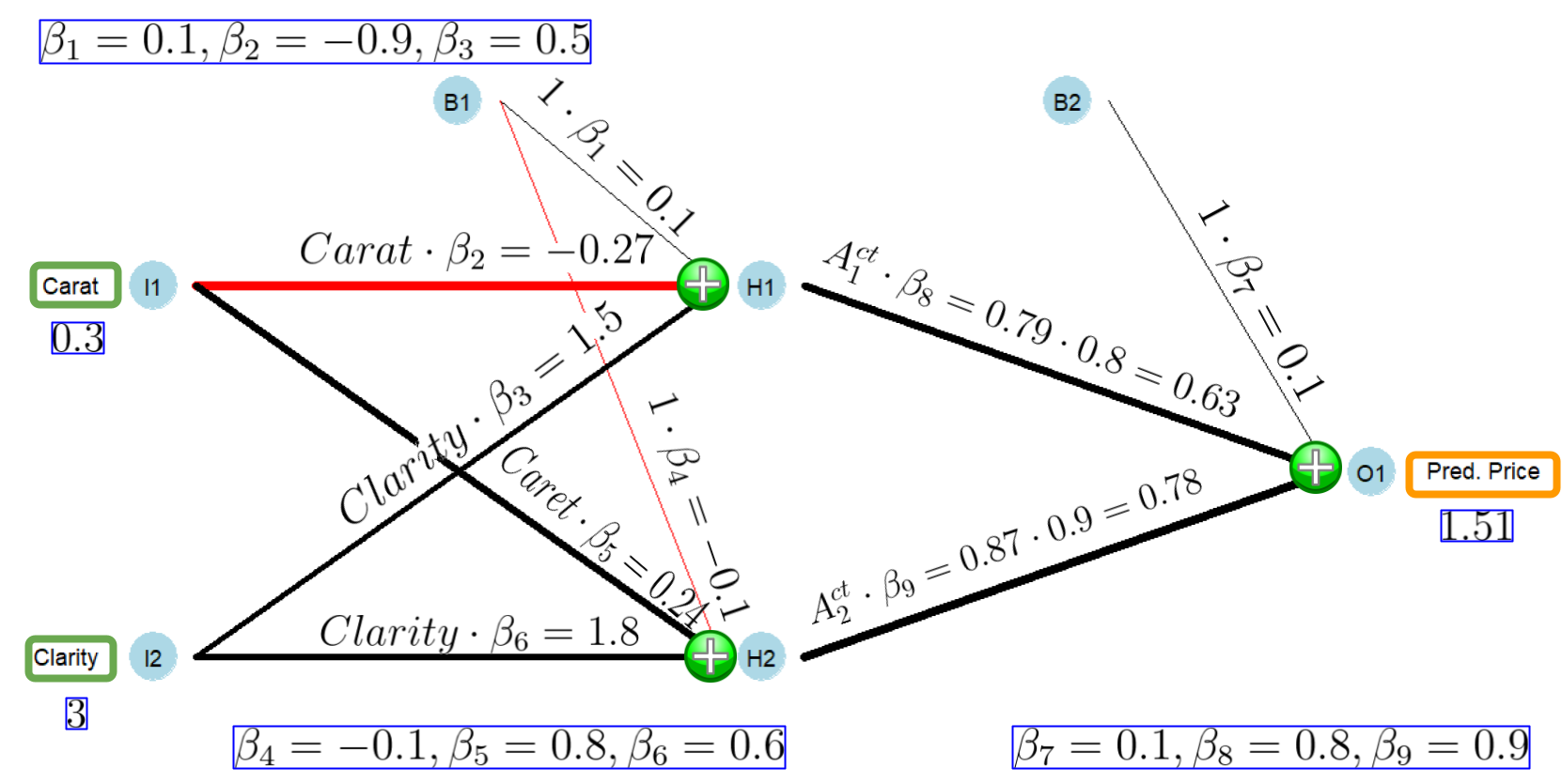
FIGURE 9.2: Graphical Representation of a Fitted Neural Network Structure

Starting in the very left in Figure 9.2, you can see that the input neurons \(I1\) and \(I2\) hold the predictor values for the diamond, \(0.3\) and \(3\), respectively. Both input values are transmitted to the hidden neuron \(H1\) and weighted with \(\beta_2\) and \(\beta_3\), resulting in values of \(0.3\cdot (-0.9)=-0.27\) and \(3\cdot 0.5=1.5\), respectively. In addition, the weighted value from the bias neuron \(B1\) \((1\cdot\beta_1=0.1)\) also arrives at the hidden neuron \(H1\). These three values are aggregated (added up) to the effective input of hidden neuron \(H1\):

\[I_{1,i}^{eff}=\underbrace{1 \cdot 0.1}_{1 \cdot \beta_1=0.1}+\underbrace{0.3\cdot(-0.9)}_{Carat_i\cdot \beta_2=-0.27}+\underbrace{3\cdot 0.5}_{Clarity_i \cdot\beta_3=1.5}=1.33\]

The effective input for the hidden neuron \(H2\) is calculated similarly, except that \(Carat_i\) is weighted with \(\beta_5\), \(Clarity_i\) is weighted with \(\beta_6\), and the value from the bias neuron \(B1\) is weighted with \(\beta_4\). Adding up these value leads to the effective input for the hidden neuron \(H2\):

\[I_{2,i}^{eff}=\underbrace{1 \cdot (-0.1)}_{1 \cdot \beta_4=-0.1}+\underbrace{0.3\cdot 0.8}_{Carat_i\cdot \beta_5=0.24}+\underbrace{3\cdot 0.6}_{Clarity_i \cdot\beta_6=1.8}=1.94\]

The effective inputs (\(I_{1,i}^{eff}\) and \(I_{2,i}^{eff}\)) together with the logistic activation functions (see Equations (9.1) and (9.2)) are used to calculate the activities (\(A^{ct}_{1,i}\) and \(A^{ct}_{2,i}\)) for the hidden neurons:

\[\begin{eqnarray*} A^{ct}_{1,i}&=&\frac{1}{1+e^{-I_{1,i}^{eff}}}\\ A^{ct}_{1,i}&=& \frac{1}{1+e^{-1.33}}=0.79\\ \\ A^{ct}_{2,i}&=&\frac{1}{1+e^{-I_{2,i}^{eff}}}\\ A^{ct}_{2,i}&=&\frac{1}{1+e^{-1.94}}=0.87 \end{eqnarray*}\]

Now that we know the activities for the hidden neurons \(H1\) and \(H2\), we can weigh them with \(\beta_8\) and \(\beta_9\), respectively (see Figure 9.2). Then we add up the weighted activities together with the bias \(B2\) according to Equation (9.7) and we get the predicted price (\(\widehat {Price}_i\)) for the diamond from Table 9.1:

\[\begin{eqnarray*} \widehat {Price}_i &=&\beta_7 + \beta_8 A^{ct}_{1,i} + \beta_9 A^{ct}_{2,i}\\ \widehat {Price}_i &=& 0.1+0.8\cdot 0.79+0.9 \cdot 0.87 = 1.51 \end{eqnarray*}\]

The prediction (obviously) does not change if we use the prediction Equation (9.8). We can show this in two steps. First, we plug the numerical \(\beta\) values into the prediction Equation (9.8):

\[\begin{eqnarray*} \widehat{P_i}&=&0.1+ \overbrace{ \frac{1}{1+e^{-(\require{color}\colorbox{sandyellowcl}{$0.1 -0.9 Carat_i+0.5 Clarity_i$})}} }^{\mbox{Activity of Hidden Neuron 1}}\cdot 0.8 \\ \nonumber \\ &+&\overbrace{ \frac{1}{1+e^{-(\require{color}\colorbox{sandyellowcl}{$-0.1 +0.8 Carat_i+0.6 Clarity_i$})}} }^{\mbox{Activity of Hidden Neuron 2}}\cdot0.9 \end{eqnarray*}\]

Next, we substitute \(Carat_i\) and \(Clarity_i\) with the values from Table 9.1 (\(0.3\) and \(3\), respectively):

\[\begin{eqnarray*} 1.51&=&0.1+ \overbrace{ \frac{1}{1+e^{-(\require{color}\colorbox{sandyellowcl}{$0.1 -0.9 \cdot 0.3 +0.5 \cdot 3$})}} }^{\mbox{Activity of Hidden Neuron 1}}\cdot 0.8 \\ \nonumber \\ &+&\overbrace{ \frac{1}{1+e^{-(\require{color}\colorbox{sandyellowcl}{$-0.1 +0.8 \cdot 0.3 +0.6 \cdot 3$})}} }^{\mbox{Activity of Hidden Neuron 2}}\cdot0.9 \end{eqnarray*}\]

Note the effective inputs are highlighted for better readability.

The predicted price for the diamond is again $1.51. Don’t get your hopes up, you won’t find a diamond for that little money.

As Table 9.1 shows, the actual price of the diamond is $506 (\(Price=506\)). The high prediction error (an underestimation of $504.49) should not surprise us because we randomly chose the \(\beta\) parameters.

At this point, we can summarize: With the \(\beta\) values given, we are able to create a prediction for any observation — including all observations from the training dataset. Since we also know the actual price for the observations, we can calculate the (squared) error for any observation in the training dataset.

For example, the squared prediction error for the observation from Table 9.1 is:

\[\begin{eqnarray*} Error_i^2&=&(\widehat{Price}_i-Price_i)^2 \\ &=&(1.51-506)^2=254510.20 \end{eqnarray*}\]

If we can use the Neural Network to generate a prediction for each of the observations from the training dataset and consequently can calculate the squared error for each of these observations, we can calculate the Mean Squared Error \((MSE)\) for the training data — for any given set of \(\beta\) values. This raises the question:

How can we iteratively change the \(\color{rubineredcl}\beta s\) to gradually improve the Neural Network’s predictive quality — minimizing the MSE?

This is what we will cover in the following section.

9.4.4 How the Optimizer Improves the Parameters in a Neural Network

For most regression⁶⁴ tasks, the Optimizer in a Neural Network (integrated in the tidymodels workflow) aims to minimize the \(MSE\)⁶⁵ by adjusting the \(\beta\) values.

To give you a basic idea of how the Optimizer adjusts the \(\beta\) values, we will use the first iteration (the first adjustment of the \(\beta\) values) as an example. We start with the randomly chosen \(\beta\) values (see Section 9.4.3) and show how the Optimizer changes these values to get a slightly lower \(MSE\). This process can then be iteratively repeated until the \(MSE\) is reasonably low.

So, let us assume the following \(\beta\) values are already randomly chosen at the beginning of the adjustment process:

\[\beta_1 = 0.1, \beta_2=-0.9 ,\beta_3=0.5 ,\beta_4 = -0.1, \beta_5 = 0.8, \beta_6 =0.6 ,\] \[\beta_7 =0.1 ,\beta_8 = 0.8,\beta_9 = 0.9\] Then we can use the definition of the \(MSE\) in connection with prediction Equation (9.8) to calculate the \(MSE\) for the initial set of \(\beta s\) for the training dataset. This \(MSE\) will be the benchmark when the Optimizer adjusts the \(\beta s\) to produce a new set of \(\beta s\) that (slightly) improves the \(MSE\). For the set of randomly chosen \(\beta\) parameters, the equation to calculate the \(MSE\) is:

\[\begin{eqnarray} MSE&=& \frac{\sum^N_{i=1}(\widehat{Price}_i - Price_i)^2}{N} \tag{9.9} \\ && \nonumber\\ \mbox{with: } && \nonumber\\ \widehat{Price}_i&=&0.1 + \overbrace{ \frac{1}{1+e^{-(\require{color}\colorbox{sandyellowcl}{$0.1 -0.9 Carat_i+0.5 Clarity_i$})}} }^{\mbox{Activity of Hidden Neuron 1}}\cdot 0.8 \nonumber \\ \nonumber \\ &+&\overbrace{ \frac{1}{1+e^{-(\require{color}\colorbox{sandyellowcl}{$-0.1 +0.8 Carat_i+0.6 Clarity_i$})}} }^{\mbox{Activity of Hidden Neuron 2}}\cdot0.9 \nonumber \end{eqnarray}\]

Note the effective inputs are highlighted for better readability.

We start with using the prediction equation to calculate the predicted price for the first observation in the training dataset \((\widehat{P_1})\). Since we know the true price \((P_1)\) for this diamond from the training data, we can calculate the related squared error as \((\widehat{P_1} - P_1)^2\).

Continuing with the other observations, we calculate the predicted price and the related squared error for the complete training dataset and then calculate the mean from all squared errors. This gives us the \(MSE\) for the training dataset related to the initial set of \(\beta s\). This calculation shows again:

For a given training dataset, we can calculate the MSE for any set of chosen \(\color{rubineredcl}\beta\) values.

Next, we increase only \(\beta_1\) by a very small amount, leaving all other \(\beta\) values unchanged, and calculate the new \(MSE\) using Equation (9.9). Consequently, the \(MSE\) will either decrease or increase compared to the benchmark \(MSE\). This provides us with information in which direction \(\beta_1\) should be changed. If increasing \(\beta_1\) was successful and the \(MSE\) decreased, mark \(\beta_1\) to be increased. Otherwise, mark \(\beta_1\) for a decrease.

Next, we reset the value for \(\beta_1\) and use the same procedure for \(\beta_2\) to find out if \(\beta_2\) should be increased or decreased.

We do the same for all other \(\beta\) parameters, and consequently, we will know for each \(\beta\) parameter if it should be increased or decreased.

The amount of the actual increase or decrease for each of the \(\beta\) parameters is proportional to the change of the \(MSE\) they triggered when individually changed. In addition, to ensure that the changes are not too large, we multiply these changes with a learning rate — a constant number smaller than one, for example, \(0.01\).⁶⁶

This procedure results in a new set of \(\beta s\) with a slightly smaller \(MSE\). This new set of \(\beta s\) becomes the new benchmark and the procedure above is repeated.

After each iteration (also called epoch), the \(MSE\) slightly improves. We continue until the \(MSE\) is lowered to the desired level or until a preset number of epochs is reached.

The process described above would work in most cases but is inefficient. In reality, the Optimizer uses a more sophisticated algorithm based on the Steepest Gradient Descent algorithm (sometimes called the Back Propagation algorithm). The Steepest Gradient Descent algorithm follows the ideas outlined above but utilizes calculus (i.e., partial derivatives) to estimate the change of the \(MSE\) when a specific \(\beta\) value is changed.⁶⁷

9.5 Build a Simplified Neural Network Model

Now it is time to see a Neural Network in action. This section uses the R nnet package (Venables and Ripley (2002)) to show a real-world application for Neural Networks. In what follows, we will emphasize the outstanding approximation properties of Neural Networks but also show how susceptible Neural Networks are to overfitting.

We use the nnet package in this section, although more advanced packages such as PyTorch have been recently implemented into R. You will use PyTorch in the interactive Section 9.7.

The reason to use nnet here is to stay compatible with Section 9.4. That is, the nnet package supports Sigmoid activation functions. In contrast, PyTorch only supports more advanced activation functions such as Rectified Linear Activation Unit (ReLU) functions (more about ReLU in Section 9.7).

As before, we start with loading the data and generating training and testing data:

library(tidymodels); library(janitor)
set.seed(777)
DataDiamonds=diamonds |>
             clean_names("upper_camel") |>
             select(Price, Carat, Clarity) |>
             mutate(Clarity=as.numeric(Clarity)) |>
             sample_n(500)

Split005= initial_split(DataDiamonds, prop=0.05)
DataTrain=training(Split005)
DataTest=testing(Split005)

As you can see, we use only \(500\) observations from the diamond dataset and assign only \(25\) observations (prop=0.05; 0.05\(\cdot\)500=25) to the training dataset. A training dataset with 25 observations is extremely small for a Neural Network application, but it is well suited to demonstrate the overfitting problem later on.

Next, we define the recipe(). It will later be added to a workflow() for the analysis:

RecipeDiamonds=recipe(Price~., data=DataTrain) |>
               step_normalize(all_predictors())

As you can see, we normalize the predictor variables. Most Neural Network applications require scaling of the predictor variables. Why this is the case is explained with the help of Figure 9.3 and in the info box that follows.

FIGURE 9.3: The Sigmoid Function

Why Neural Networks Need Scaled Predictors

When some or all predictor variables contain large values, the effective inputs can also become large. Suppose one of the inputs is the U.S. Gross Domestic Product (\(GDP\)) measured in millions of U.S. Dollars (e.g., $26,860,000 million for 2022). Such high values multiplied by the related \(\beta\) values will be an additive part of the effective inputs for the hidden neurons. Consequently, these effective inputs will also become large even if the absolute \(\beta\) values that multiply the \(GDP\) are small (e.g., \(0.004\) or \(-0.0002\)).

You can see the resulting problem in Figure 9.3. Effective inputs smaller than \(-5\) or greater than \(5\) will impact the activation function at its (almost) horizontal sections, leading to activity values of either \(0\) or \(1\).

Consequently, for predictor variables with large input values such as the \(GDP\), a Neural Network will likely create activities of either \(0\) or \(1\) for all observations. Afterward, between the hidden and the output layer (see Figure 9.1), these \(0\) or \(1\) activities will be multiplied with the related \(\beta\) values but because the activities do not change for the different observations (they stay \(0\) or \(1\)), the output of the Neural Network will be constant regardless of which observation is processed.

If this is not bad enough, the optimization process used in Neural Networks (most of the times a variation of the Steepest Gradient Descent algorithm) has difficulties changing the \(\beta s\) when the slope of the activation functions is \(0\). Consequently, the \(\beta s\) that multiply the inputs would not change (get smaller) during the iterations.⁶⁸ The training process gets stuck.

To see a numerical example, you can process two very different diamonds through the Neural Network in Figure 9.2 (\(Carat_1=0.1\), \(Clarity_1=5\) and \(Carat_2=0.4\), \(Clarity_2=6\)). Both diamonds will generate \(A^{ct}_1=A^{ct}_2=1\) and thus, despite being different, will have exactly the same predicted price.

As a rule of thumb: When you get the same or very similar predictions for all or most of your training data, it is often due to a lack of scaling or inappropriate scaling.

In the recipe above, we used step_normalize() and thus applied Z-score Normalization (see Section 4.6 for more details). The Z-score Normalization scaling method is often used for Neural Networks. Z-score Normalization is unlikely to produce values smaller than \(-5\) or greater than \(5\).⁶⁹ Additionally, the scaled inputs are multiplied by absolute \(\beta\) values smaller than one. Consequently, effective input values are not large and have a good chance to impact the activation function at different points in the middle section. In this section the slope is not zero and the generated activities discriminate between different input values (see Figure 9.3). Consequently, the Neural Network generates different outputs for different observations.

Next, we create a model design for the Neural Network analysis:

ModelDesignNN= mlp(hidden_units=50, epochs=10000, penalty=0) |> 
               set_engine("nnet") |>
               set_mode("regression") 

The model command for an MLP network is mlp(), and we use the nnet package (see set_engine("nnet")). The argument hidden_units=50 determines that we use a hidden layer with 50 hidden neurons, epochs=10000 determines that the Optimizer runs 10,000 epochs (iterations), and penalty=0 determines that we do not use regularization. The package nnet supports regularization similar to \(Ridge\) regularization, and the value assigned to penalty determines how the penalty term and the \(MSE\) are weighted in the target function. All three arguments can optionally be tuned by assigning tune(). Here, we keep it simple and do not tune the Neural Network, but in the interactive Section 9.7, you will tune a Neural Network using PyTorch.

To fit a workflow() model with the training data, we must add the recipe and the model design to a workflow and use the built-in Optimizer and the training data (fit(DataTrain)) to find optimal parameters for the \(\beta s\):

WFModelNN=workflow() |> 
          add_model(ModelDesignNN) |> 
          add_recipe(RecipeDiamonds) |> 
          fit(DataTrain)

Since the workflow WFModelNN is now a fitted workflow, we can use it for predicting diamond prices.

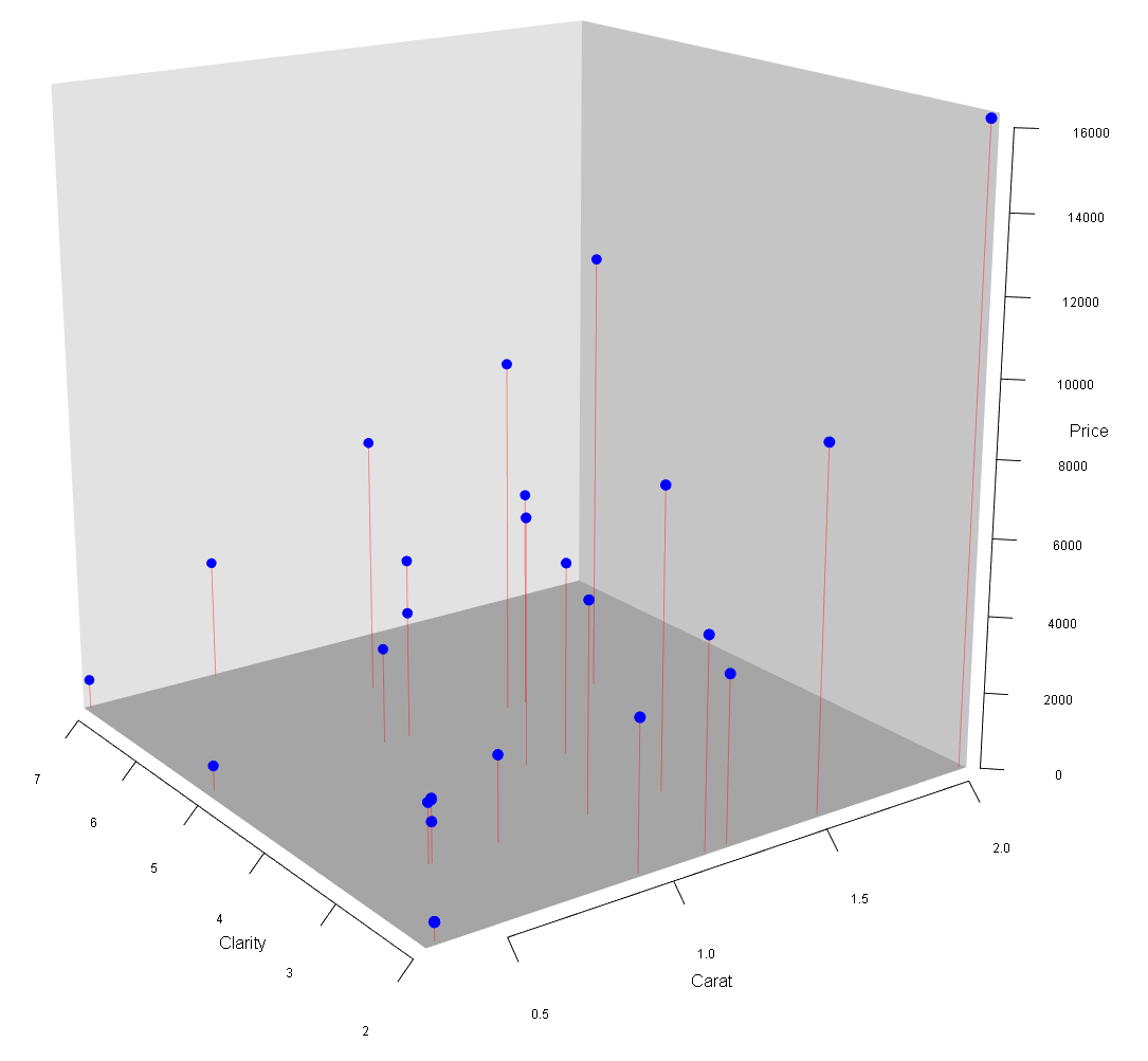
FIGURE 9.4: 3D Scatter Plot for the Diamonds Data

We start with generating predictions for the training dataset and evaluating how well the predictions approximate the true prices in the training dataset. Again, we use the augment() command to create the predictions. These predictions are then augmented to the training dataset by creating an extra column named \(.pred\). The resulting data frame is saved as DataTrainWithPred.

The metrics() command then compares for each observation the prediction \((.pred)\) with the true value for the diamond price \((Price)\) and calculates the root of the mean squared error \(\sqrt{MSE}\), \(r^2\) and the mean absolute error \((mae)\) for the training data:

DataTrainWithPredNN=augment(WFModelNN, new_data=DataTrain) 
metrics(DataTrainWithPredNN, truth=Price, estimate=.pred)

## # A tibble: 3 × 3
##   .metric .estimator .estimate
##   <chr>   <chr>          <dbl>
## 1 rmse    standard     198.   
## 2 rsq     standard       0.996
## 3 mae     standard     111.

As you can see, the Neural Network approximates the training data extremely well. For example, \(r^2=0.996\).

How such a (suspiciously) good approximation is possible, is illustrated in Figures 9.4 and 9.5. In Figure 9.4, you can see a 3D scatter plot of the training data. The two axes on the bottom of the 3D cube reflect \(Carat\) and \(Clarity\) for each diamond. The height of each data point (visualized by the red line) depicts the \(Price\) for each diamond.

The prediction goal for the Neural Network is to find a surface that approximates these points as well as possible.

Because of the high number of iterations (epochs=10000) and the high degree of non-linearity of the Neural Network (50 hidden neurons with non-linear logistic functions and \(201\) parameters), the Neural Network can produce a very flexible prediction surface.

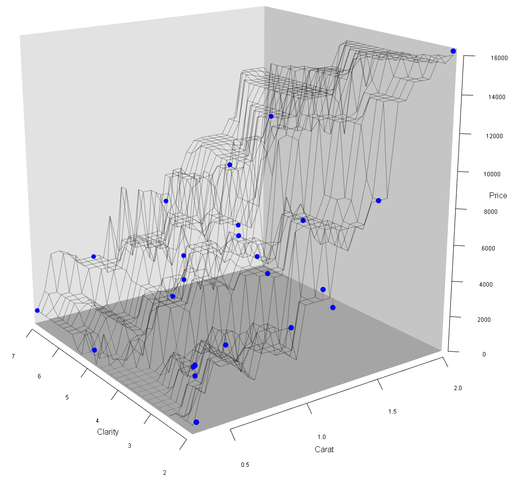
FIGURE 9.5: Diamond Data and Prediction Surface

Figure 9.5 shows that the fitted Neural Network workflow model generates a prediction surface that almost perfectly approximates the training data. This prediction surface bends in many ways to make the close approximation possible. This high flexibility of the prediction surface (i.e., the underlying prediction function) was made possible by the high number of hidden neurons leading to a total of \(201\) \(\beta\) parameters.

A Neural Network with a sufficiently large number of hidden neurons can take the form of a highly non-linear surface to approximate training data almost perfectly. In fact, a “\((\dots)\) standard multilayer feedforward network architecture using arbitrary squashing functions can approximate virtually any function of interest to any desired degree of accuracy, provided sufficiently many hidden units are available” (Hornik, Stinchcombe, and White (1989)).

To intuitively understand the outstanding approximation ability of a Neural Network, consider that a Neural Network consists of many hidden neurons and thus of many Sigmoid functions. Sigmoid functions are squashing functions because they squash all input values between two output values (\(0\) and \(1\) in the case of the Logistic function). As Figure 9.3 shows, each Sigmoid function forms a step similar to a step in a staircase. Although smoother than a staircase step, a Sigmoid function, like a staircase step, is flat first, then upward (or possibly downwards), and finally flat again.

Changing the \(\beta\) values that impact the effective input \(j\) \((I^{eff}_{j,i})\) of a specific Sigmoid activation function and changing the \(\beta\) value that weighs the resulting activity \((\beta_jA^{ct}_{j,i})\), can move a step (Sigmoid function) horizontally, increase or decrease the step size, change the steepness, and also convert a step from an upward to a downward step.

Since a Neural Network consists of many hidden neurons, many Sigmoid (steps) functions can be combined to a staircase-like structure with smaller and bigger steps as well as upwards and downward steps — depending on the \(\beta\) parameter values. This staircase-like structure — if it has enough steps — can approximate a function in any given range to any degree.

The mathematical formula behind this staircase-like structure is the Neural Network prediction function. It combines the Sigmoid (steps) functions to approximate whatever continuous function needs to be approximated (in a given range) with various up- and downward steps.

Consequently, with this procedure, a Neural Network can approximate a given function to any degree of smoothness in a given range by increasing the number of hidden neurons.

FIGURE 9.6: Three Sigmoid Functions Approximate a Sine Function

Figure 9.6 shows an example of the arguments outlined above. The goal is to approximate a sine function (see the orange dots in the upper diagram in Figure 9.6) in an input range between 0 and 9 with a Neural Network. The sine function to be approximated is:

\[ y_i=\sin(x_i+5)+1 \]

We use a Neural Network with one input \((x_i)\), three hidden neurons with Logistic activation functions, and one output \(\widehat{y_i}\).

When all \(\beta\) values are appropriately chosen,⁷⁰ the three \(\beta\) weighted activation functions of the three hidden neurons form three steps (see the lower three diagrams in Figure 9.6). When these steps are combined (added up) together with the bias for the output neuron \((\beta_{10}=2)\) they form the Neural Network prediction function (see the blue line in the upper diagram of Figure 9.6). As you can see, we get a good approximation of the sine function. The Neural Network prediction function forms a staircase-like structure with one step up, one step down, and one step up (see the blue line in the upper diagram of Figure 9.6). If we want to increase the smoothness of the approximation, we could work with six hidden neurons (six steps). With appropriate values for the \(\beta\) parameters, we could form a staircase-like structure with two (smaller) steps up, two (smaller) steps down, and two (smaller) steps up.

You can find a link to a related blog post and a simulation app that allows you to interactively adjust the \(\beta\) values for the Neural Network from Figure 9.6 in the Digital Resource Section 9.9.

It is important to mention that the procedure above is more like a proof of concept rather than a real proof. The procedure shows only one way a Neural Network can possibly approximate a function. It is not likely that the \(\beta\) parameters determined by the Optimizer will actually form a staircase-like structure. Also, the mathematical proof from Hornik, Stinchcombe, and White (1989) is different and more advanced.

Now that we know that Neural Networks with enough hidden neurons can approximate any training dataset to a very high degree, the crucial question is, how well our fitted Neural Network can predict the testing data — data the Neural Network has never seen before.

In the code block below, we use the augment() and the metrics() commands as above when evaluating training data performance, except that we now evaluate the testing data (DataTest):

DataTestWithPredNN=augment(WFModelNN, new_data=DataTest)
metrics(DataTestWithPredNN, truth=Price, estimate=.pred)

## # A tibble: 3 × 3
##   .metric .estimator .estimate
##   <chr>   <chr>          <dbl>
## 1 rmse    standard    2202.   
## 2 rsq     standard       0.709
## 3 mae     standard    1273.

The prediction result is not good. For instance, for the testing data, the \(mae\), the amount our model on average over/underestimates a diamond’s price, is $1,273. This is a typical case of overfitting; the training data approximation is good \((mae=110.94)\), but the prediction quality based on the testing data is poor.

Neural Networks with a large number of parameters are prone to overfitting, especially when the training dataset is relatively small.

Section 9.7 will guide you through an interactive project where you can tune a Neural Network to avoid overfitting. You will use the diamonds dataset and utilize all four diamond appraisal Cs (\(Carat\), \(Clarity\), \(Cut\), and \(Color\)) as predictor variables. You will also use PyTorch with the brulee package instead of nnet.

9.6 NNet vs. PyTorch (brulee)

PyTorch is a machine learning framework initially developed by Facebook (now Meta AI). Since 2022, it is curated by the Linux Foundation. PyTorch was for a long time only accessible through Python, but in 2021, the developers of tidymodels created the R package brulee (Kuhn and Falbel (2022)), which makes some of the functionality from PyTorch available to tidymodels. This includes an MLP network implementation.

In this section, we will discuss some of the differences between a Neural Network created with the nnet package and a Neural Network created by PyTorch (via the brulee package).

The nnet package (Venables and Ripley (2002)) was one of the earliest R packages to support Neural Networks. It is well suited for educational purposes, especially to demonstrate how Neural Networks can be used for predictions and to display Neural Networks as graphs.⁷¹

In contrast, PyTorch is an advanced data science toolkit, and its Neural Network functionality is more up-to-date. Some of PyTorch’s functionality, including support for MLP networks was recently included in R through the brulee package.

There are quite a few differences between MLP networks supported by nnet and by PyTorch. In this section, we will focus on two aspects:

Hyper-Parameters:

In PyTorch, you can set and tune numerous hyper-parameters that are either unavailable in nnet or are available, but not as advanced. For example, in nnet, you can tune the number of hidden neurons for one hidden layer. In PyTorch, you can set and tune the number of hidden neurons for multiple hidden layers.

Activation Functions: PyTorch allows us to use the Rectified Linear Unit (ReLU) activation function, while nnet does not support ReLU activation function. In what follows, we will introduce how ReLU functions work and why they are superior to classical Sigmoid activation functions, which are supported in nnet.

9.6.1 Hyper-Parameters

Below is a selective list of hyper-parameters that PyTorch supports. The list is limited to the hyper-parameters that we will later use in the interactive Section 9.7.

epochs=

Determines the maximum number of epochs used by the Optimizer for training. Internally PyTorch generates a validation dataset and if the prediction error does not improve for five consecutive epochs, it stops the training even if the maximum number of epochs set by epochs= has not been reached.

hidden_neurons=

This hyper-parameter determines the number of hidden neurons and, at the same time, the number of hidden layers. When working with only one hidden layer like here, you can assign a number to hidden_neurons=, which determines the number of neurons for the only hidden layer (e.g., hidden_neurons=50 for 50 neurons in the only hidden layer).

Suppose you would like to work with more than one layer. In that case, you must assign a vector to hidden_neurons= where each element determines the number of hidden neurons for consecutive hidden layers (e.g., hidden_neurons=c(25,30,20) for a Neural Network with three layers where the first layer consists of 25 neurons, the second layer of 30 neurons, and the third of 20 neurons).

dropout=

PyTorch allows randomly switching off a predefined percentage of hidden neurons for each iteration of the Optimizer process. The value assigned to dropout determines the proportion of hidden neurons randomly switched off at each iteration. For example, dropout=0.25 indicates that the Optimizer randomly switches off 25% of the hidden layer’s neurons at each iteration of the training process.

penalty=

Determines the weight of the penalty term compared to the \(MSE\) in the target function when regularization is used (see Chapter 7 for details). By default Ridge regularization is used with penalty=0.001.

9.6.2 ReLU Activation Functions

Unlike the nnet package, PyTorch supports ReLU activation functions. In this section, we will discuss ReLU activation functions and focus on:

1. Introducing the ReLU activation function.

2. Demonstrating that Neural Networks with ReLU activation functions has the same outstanding approximation properties as a Neural Networks with Sigmoid activation functions.

3. Discussing the problem of the Vanishing Gradient in context of classical Sigmoid vs. ReLU activation functions. A Vanishing Gradient can lead to a situation where the Optimizer cannot change the \(\beta\) parameters anymore, although they are still far from optimal.

Let us start with how a ReLU activation function determines the activity of a hidden neuron:

\[\begin{eqnarray} Act_{j,i}&=&max\left (0, I_{j,i}^{eff}\right ) \tag{9.10}\\ &&\mbox{with $j: =$ hidden neuron number and $i:=$ observation number} \nonumber \end{eqnarray}\]

Equation (9.10) shows the algebraic form of a ReLU activation function. If the effective input is greater than \(0\), the ReLU function returns the effective input as activity \((Act_{j,i}=I_{j,i}^{eff})\). If the effective input is smaller than \(0\), the ReLU function returns \(0\) \((Act_{j,i}=0)\). You also can see this in Figure 9.7 below. For all positive effective inputs, we get the Linear-Parent-Function graph (y=x-graph). For all negative values we get a straight line with \(y=0\).

Figure 9.7 shows, that the graph of the ReLU activation function is limited to depicting only half of a step. In contrast, the graph of a Sigmoid activation function depicts a full step. Therefore the question arises if Neural Networks with ReLU activation functions have the same outstanding approximation properties as Neural Networks with Sigmoid activation functions?⁷²

FIGURE 9.7: The ReLU Activation Function

The answer is that ReLU activation functions do have the same outstanding approximation properties. This is because we can combine two ReLU functions into a complete step, and then they have the same approximation properties as classical Sigmoid (full-step) functions.

We can show this with an example by using a Neural Network with one predictor variable \((x)\), one hidden layer, and multiple hidden neurons.

Let us look at the first hidden neuron. Before its activity is transmitted to the output neuron it is weighted with \(\beta_3\). Therefore we consider \((\beta_3 Act_{1,i})\) rather than its activity \((Act_{1,i})\) alone:

\[\begin{equation} \beta_3Act_{1,i}=\beta_3 \cdot max\left (0, I^{eff}_{1,i}\right ) \tag{9.11} \end{equation}\]

Since we have only one predictor variable \(x\), substituting the resulting effective input \(I_{1,i}^{eff}=\beta_1+\beta_2 x_i\) into Equation (9.11) leads to:

\[\begin{eqnarray} \beta_3 Act_i&=&\beta_3 max\left (0, \beta_1 +\beta_2 x_i \right ) \tag{9.12} \\ \mbox{with:}&& \beta_1 \mbox{: parameter for bias neuron $B1$ and} \nonumber \\ && \beta_2 \mbox{: parameter for the only predictor variable $x$} \nonumber \end{eqnarray}\]

Equation (9.12) can be plotted and for \(\beta_1=0\), \(\beta_2=1\), and \(\beta_3=1\), the plot resembles the ReLU from Figure 9.7.

By changing the \(\beta\) parameters \(\beta_1\), \(\beta_2\), and \(\beta_3\) the graph of the augmented ReLU function in Figure 9.7 can be transformed:

• horizontally shifted (by changing \(\beta_1\))

• the slope can be changed (by changing \(\beta_3\))

• the graph can be turned upside down (by changing \(\beta_3\) to a negative value)

• the graph can be mirrored horizontally (by changing the sign of \(\beta2\))

When using the transformations above on two different augmented ReLU functions (two hidden neurons) they can jointly form a step function similar to a Sigmoid function, except that the step based on the two ReLU function has two kinks and the slope between the two kinks is constant.

In Section 9.9, we provide a link to an Internet app and a related blog post where you can transform and combine two ReLU functions to form a complete step function.

In summary: If we can combine two hidden neurons with ReLU activation functions into a complete step function, we can expect the same approximation properties from a Neural Network with ReLU activation functions that we derived in Section 9.5 for Neural Networks with Sigmoid functions.

The constant slope of a ReLU activation function is a major advantage over a Sigmoid function. Let us compare the slope of the Logistic activation function in Figure 9.3 with the slope of the ReLU activation function in Figure 9.7. The ReLU activation function has a constant slope of one for all positive effective inputs. In contrast, the slope of the Logistic activation function is always smaller than one, and it becomes very small when the effective input gets greater in absolute terms (when approaching the red and blue lines in Figure 9.3).

While the small slope of Logistic activation functions is not a problem for Neural Networks with one layer, it is a problem for Neural Networks with many layers.

When the Optimizer adjusts individual \(\beta\) values in a multi-layer Neural Network and calculates by how much they change from iteration to iteration, the weighted slopes of the activation functions in different layers are multiplied.⁷³ If these weighted slopes are smaller than one, each multiplication makes the change of the related \(\beta\) smaller. With enough layers, the calculated change might get close to zero. Consequently, the \(\beta\) parameters will not change anymore, and the optimization process gets stuck. This problem is called the Vanishing Gradient.⁷⁴

Since ReLU activation functions have a constant slope of one for positive effective inputs, the Vanishing Gradient problem is mostly mitigated when using ReLU activation functions.

In the following interactive Section 9.7, you will work with a Neural Network with ReLU activation functions. You will tune a Neural Network and estimate diamond prices.

9.7 🧭Using PyTorch to Predict Diamond Prices

Interactive Section

In this section, you will find content together with R code to execute, change, and rerun in RStudio.

The best way to read and to work with this section is to open it with RStudio. Then you can interactively work on R code exercises and R projects within a web browser. This way you can apply what you have learned so far and extend your knowledge. You can also choose to continue reading either in the book or online, but you will not benefit from the interactive learning experience.

To work with this section in RStudio in an interactive environment, follow these steps:

1. Ensure that both the learnR and the shiny package are installed. If not, install them from RStudio’s main menu (Tools -> Install Packages \(\dots\)).

2. Download the Rmd file for the interactive session and save it in your project folder. You will find the link for the download below.

3. Open the downloaded file in RStudio and click the Run Document button, located in the editing window’s top-middle area.

For detailed help for running the exercises including videos for Windows and Mac users we refer to: https://blog.lange-analytics.com/2024/01/interactsessions.html

Do not skip this interactive section because besides providing applications of already covered concepts, it will also extend what you have learned so far.

Below is the link to download the interactive section:

https://ai.lange-analytics.com/exc/?file=10-DeepLearnExerc100.Rmd

In this section, you will use PyTorch to run and tune a Neural Network model predicting diamond prices. By default, PyTorch uses ReLU activation functions.

Tuning a Neural Network requires more computer resources than the machine learning models from the previous chapters. We implemented some restrictions to allow you to run and tune the model in a browser. Instead of using all 53,940 observations from the diamonds dataset, we will choose only 500 randomly selected observations, and we will tune only two hyper-parameters (hidden_neurons= and dropout=). In the initial setup, three values are tried out for hidden_neurons and two values for dropout.

You can change the values from the initial setup or add more values for each hyper-parameter. However, increasing the values that are tried out for each of the hyper-parameters, will also increase the execution time for the tuning process (the maximum computing time available in a browser is currently set to 30 minutes). Please consider, with such a long execution time and R running in a browser, the tuning process might become unstable, and the browser might crash.

If you need more computing time to tune more hyper-parameters with more values or you plan to use all 53,940 observations from the diamonds dataset, we provide an alternative. You can download an R script with similar code as here without computing time restrictions. The R script runs in RStudio and you can run the tuning for several hours overnight. You find a link and a short description for this R script in the Digital Resource Section 9.9.

By default, the R script utilizes the complete diamonds dataset. Since computing time is only limited by your patience, you can try out more values for the pre-set hyper-parameters (hidden_neurons= and dropout=), and you can add different hyper-parameters such as penalty=tune() to try out various degrees of regularization.

Let us now go to the Neural Network that you will run in a browser. You will estimate the price of diamonds with a Neural Network under real-world conditions:

1. You will use all big C variables \(Carat\), \(Clarity\), \(Cut\), and \(Color\) as predictor variables. We used \(Carat\) and \(Clarity\) already in Section 9.5. Here, the variables \(Cut\) and \(Color\) are added to the analysis. \(Cut\) describes the quality of the cut of a diamond and is rated from 1 (lowest) to 6 (highest). \(Color\) rates the color of a diamond from 1 (highest) to 7 (lowest); note the opposite direction of the rating scale.

2. As already explained in Section 9.6, you will use the more advanced PyTorch Neural Network from the brulee package instead of the Neural Network from the nnet package.

3. You will tune the Neural Network’s hyper-parameters (hidden_units and dropout) by using Cross-Validation.

Keep in mind that you have to install the brulee package before you can execute the code. After the brulee package is installed, the PyTorch software must also be installed. This is straightforward: When the package is used for the first time (i.e., with library(brulee)) a popup window asks to download and install the required software. After confirming with “Yes”, the PyTorch software will be installed.

We again use the 10-Step Template introduced in Section 6.6. Steps 1 – 4 are already prepared for you.

Step 1 - Generate Training and Testing Data:

library(tidymodels); library(janitor); library(brulee)
set.seed(888)
DataDiamonds=sample_n(diamonds, 500) |>
             clean_names("upper_camel") |>
             select(Price, Carat, Cut, Color, Clarity) |> 
             mutate(Cut=as.integer(Cut), Color=as.integer(Color),
                    Clarity=as.integer(Clarity))
set.seed(888)
Split70=initial_split(DataDiamonds, prop=0.7, strata=Price, breaks=5)
DataTrain=training(Split70)
DataTest=testing(Split70)

In the code block above, we load the data and choose randomly 500 observations. Then we select the outcome variable \((Price)\) and the predictor variables \(Carat\), \(Clarity\), \(Cut\), and \(Color\) transforming the factor-levels of the last three variables to numerical integer values. Finally, we split the data into training and testing data.

Step 2 - Create a Recipe:

We use the same recipe() command as in Section 9.5:

RecipeDiamonds=recipe(Price~., data=DataTrain) |>
               step_normalize(all_predictors())

Again, we use step_normalize() for Z-score Normalization ⁷⁵ of all predictors. As explained in Section 9.5, the predictor variables for a Neural Network need to be scaled. Otherwise, the Optimizer likely will not generate suitable \(\beta\) values.⁷⁶

Step 3 - Create a Model Design:

In the code block below, we create a model design. Like in Section 9.5, we use the mlp() command to create an MLP network model. However, we utilize the brulee package and therefore PyTorch rather than the nnet package (see set_engine("brulee")):

ModelDesignNN=mlp(hidden_units=tune(), dropout=tune(), 
                  epochs=100, penalty=0) |> 
              set_engine("brulee") |>
              set_mode("regression")

The hyper-parameters hidden_units and dropout are prepared for tuning (see hidden_units=tune() and dropout=tune()). The hyper-parameter penalty is set to zero (no regularization) and epochs is set to 100 (the default).

When you use the provided R script from the Digital Resource Section 9.9 to run the code in RStudio rather than in a browser, you can increase the value for epochs (e.g., epochs=1000), and you can tune other hyper-parameters. For example, you can set penalty=tune() to introduce different degrees of regularization. Remember that you have to provide the values you would like to try out for each hyper-parameter in Step 5 (Create a Hyper-Parameter Grid).

Step 4 - Add the Recipe and the Model Design to a Workflow:

Below, we add the recipe and the model design to a workflow, which will be tuned in Step 7:

TuneWFModelNN=workflow() |> 
              add_model(ModelDesignNN) |> 
              add_recipe(RecipeDiamonds)

Steps 5 – 10 in the code block below are the steps you will execute (and potentially modify).

It is recommended to execute the code below unchanged in a first attempt. Then, you can start modifying the code and see what happens. Make small changes first to see how the computing time responds on your machine. To use different values for the hyper-parameters, modify the Hyper-Parameter Grid in Step 5.

# Step 5 - Create a Hyper-Parameter Grid:
#          To try out different hyper-parameter values, change the 
#          values that are assigned to the respective hyper-parameters 
#          below.
ParGridNN=expand.grid(hidden_units=c(10, 20, 50), dropout=c(0, 0.25))

# Step 6: - Create Resamples for Cross-Validation:
#           You can change v= to consider a different
#           number of folds (e.g. v=10). Note, computing
#           time will change proportionately.
set.seed(888)
FoldsForTuningNN=vfold_cv(DataTrain, v=7, strata=Price)

# Step 7 - Tune the Workflow and Train All Models:
#  (this step requires patience; run time 5-30 minutes)
set.seed(888)
TuneResultsNN=tune_grid(TuneWFModelNN, resamples=FoldsForTuningNN,
                        grid=ParGridNN, metrics=metric_set(rmse, rsq, mae))

# Step 8 - Extract the Best Hyper-Parameter(s) 
BestHyperParNN=select_best(TuneResultsNN, metric="rmse")
print("Best Hyper-Parameters:")
print(BestHyperParNN)

# Step 9 - Finalize and Train the Best Workflow Model:
#  (this step requires a little patience; run time 1-10 minutes)
set.seed(888)
BestWFModelNN=TuneWFModelNN |>
              finalize_workflow(BestHyperParNN) |>
              fit(DataTrain)

# Step 10: Assess Prediction Quality Based on the Testing Data:
DataTestWithPredBestModelNN=augment(BestWFModelNN,DataTest)
metrics(DataTestWithPredBestModelNN, truth=Price, 
        estimate=.pred)

# Plot Validation Performance of Hyper-Parameters
autoplot(TuneResultsNN)

When you execute the code block above, the tuning process starts. It can take a while until you get a result. Depending on your computer, it can take between 5 and 30 minutes. To accommodate longer computing time in the browser, we extended the maximum computing time available to 30 minutes.

If you use the initial settings, when you execute the code above in a browser, the command autoplot(TuneResultsNN) (at the end of the code block) will create a plot similar to the one in Figure 9.8.

FIGURE 9.8: Plot and Predictions

You can see in Figure 9.8 that more hidden neurons lead to a lower mean average error, lower root mean squared error, and higher \(r^2\). Figure 9.8 also shows that a higher dropout rate leads to a higher mean average error, higher root mean squared error, and lower \(r^2\). This suggests trying more hidden neurons and lower dropout rates.

For your information, we also calculated the metrics based on the testing data in Step 10 of the template. Please keep in mind that metrics based on testing data should only be used to assess the last model and not for tuning adjustments because this could lead to overfitting.

9.8 When and When Not to Use Neural Networks

• Neural Networks shine when they consist of many layers and many hidden neurons (some Neural Networks like Natural Language Processing networks, often have millions or even billions of parameters). These networks are well suited to model highly complex non-linear relationships.

• Neural Networks with many layers and hidden neurons are also prone to overfitting if not accompanied by large datasets (see Section 9.5 for details). Even datasets with hundreds or thousands of observations might not be big enough to avoid overfitting when using large(r) Neural Networks.

  There is no rule on how many layers and how many hidden neurons a Neural Network should have. You can start with a reasonable architecture (number of hidden layers and hidden neurons) given the size of your dataset and then use tuning to find the best performing Neural Network based on Cross-Validation.

• Neural Networks with one hidden layer like in this chapter, perform well to predict relationships between multiple predictor variables and one outcome variable. However, other machine learning algorithms such as Random Forest (see Chapter 10) should also be considered since they often perform similar or better.

• Neural Networks can also predict linear relationships. However, since the \(\beta\) parameters cannot be interpreted as in linear OLS models, OLS is better suited to predict linear relationships. It is good practice to first develop a linear model as a benchmark and then evaluate if a Neural Network (or other machine learning model) can outperform it.

9.9 Digital Resources

Below you will find a few digital resources related to this chapter such as:

• Videos
• Short articles
• Tutorials
• R scripts

These resources are recommended if you would like to review the chapter from a different angle or to go beyond what was covered in the chapter.

Here we show only a few of the digital resourses. At the end of the list you will find a link to additonal digital resources for this chapter that are maintained on the Internet.

You can find a complete list of digital resources for all book chapters on the companion website: https://ai.lange-analytics.com/digitalresources.html

Neural Network Video from StatQuest

A video from StatQuest by Josh Starmer. This video is Part 1 from a series of eight videos about Neural Networks. While most of the videos exceed the scope of this book, Part 1 complements topics in the book.

Link: https://ai.lange-analytics.com/dr?a=343

How Two ReLU Functions Can Form a Complete Step Function

This is a blog post by Carsten Lange that shows how two Rectified Linear
Unit (ReLU) activation functions can be combined into a complete step function (squashing function). The post includes a simulation that allows for changing the beta values of two ReLU functions with the goal of creating a complete step function.

Link: https://ai.lange-analytics.com/dr?a=352

R Script for Tuning and Training a Neural Network to Predict Diamond Prices

Here you can download an R script to tune and train a neural network to predict diamond prices. The R script contains similar code as the related interactive section of the book. In contrast to the interactive section, the code runs in RStudio instead of a browser, and the maximum runtime is not restricted.

The R script loads the complete set of observations from the diamonds dataset, and all hyper-parameters can be tuned, The maximum number of epochs is set to 1000 and can be changed.

It is recommended that you experiment with tuning settings in the R script (see Step 5) and try to improve the cross-validation results. At the very end of the R script, you find sample tuning settings that produce relatively good results but require between one to several hours of computing time, depending on your computer. Use the sample tuning setting only after you have experimented with the tuning, and then see if your results can beat the sample tuning results.

Link: https://ai.lange-analytics.com/dr?a=354

More Digital Resources

Only a subset of digital resources is listed in this section. The link below points to additional, concurrently updated resources for this chapter.

Link: https://ai.lange-analytics.com/dr/deeplearn.html

References

Aden-Buie, Garrick, Barret Schloerke, and JJ Allaire. 2022. Learnr: Interactive Tutorials for r. https://CRAN.R-project.org/package=learnr.

Beck, Marcus W. 2018. “NeuralNetTools: Visualization and Analysis Tools for Neural Networks.” Journal of Statistical Software 85 (11): 1–20. https://doi.org/10.18637/jss.v085.i11.

Chan, Chung-Hong, Geoffrey C. H. Chan, Thomas J. Leeper, and Jason Becker. 2021. Rio: A Swiss-Army Knife for Data File i/o.

Chang, Winston, Joe Cheng, JJ Allaire, Carson Sievert, Barret Schloerke, Yihui Xie, Jeff Allen, Jonathan McPherson, Alan Dipert, and Barbara Borges. 2022. Shiny: Web Application Framework for r. https://CRAN.R-project.org/package=shiny.

Firke, Sam. 2023. Janitor: Simple Tools for Examining and Cleaning Dirty Data. https://CRAN.R-project.org/package=janitor.

Haykin, Simon. 1999. Neural Networks: A Comprehensive Foundation (2nd Edition). Prentice Hall, Upper Saddle River, NJ.

Hornik, Kurt, Maxwell Stinchcombe, and Halbert White. 1989. “Multilayer Feedforward Networks Are Universal Approximators.” Neural Networks 2 (5): 359–66. https://doi.org/10.1016/0893-6080(89)90020-8.

Kuhn, Max, and Daniel Falbel. 2022. Brulee: High-Level Modeling Functions with ’torch’. https://CRAN.R-project.org/package=brulee.

Kuhn, Max, and Hadley Wickham. 2020. Tidymodels: A Collection of Packages for Modeling and Machine Learning Using Tidyverse Principles. https://www.tidymodels.org.

Lange, Carsten. 2003. Neuronale Netze in der Wirtschaftswissenschaftlichen Prognose und Modellgenerierung (Neural Networks in Economic Modeling). Physica, Heidelberg, Germany.

Manassa, I. 2021. “Mathematics Behind Gradient Descent.” Geek Culture. https://medium.com/geekculture/mathematics-behind-gradient-descent-f2a49a0b714f.

McCulloch, Warren S., and Walter Pitts. 1943. “A Logical Calculus of the Ideas Immanent in Nervous Activity.” The Bulletin of Mathematical Biophysics 5 (4): 115–33. https://doi.org/10.1007/bf02478259.

Venables, W. N., and B. D. Ripley. 2002. Modern Applied Statistics with s. Fourth. Springer, New York, NY. https://www.stats.ox.ac.uk/pub/MASS4/.

Wang, Chi-Feng. 2019. “The Vanishing Gradient Problem. Its Causes, Its Significance, and Its Solutions.” Towards Data Science. https://towardsdatascience.com/the-vanishing-gradient-problem-69bf08b15484.

Wickham, Hadley. 2016. Ggplot2: Elegant Graphics for Data Analysis. Springer, New York, NY. https://ggplot2.tidyverse.org.

Zhu, Hao. 2021. kableExtra: Construct Complex Table with ’kable’ and Pipe Syntax. https://CRAN.R-project.org/package=kableExtra.

---

59. For example, it is believed that GPT-4 is trained on 1.7 trillion parameters.↩︎

60. All layers between the input and the output layers are called hidden layers.↩︎

61. This dataset is built into the ggplot2 R package (Wickham (2016)).↩︎

62. The following description was retrieved from the Brilliant Earth website (https://www.brilliantearth.com/diamond/buying-guide/).↩︎

63. The \(clarity\) rating in the diamonds dataset is in line with the rating categories from the Gemological Institute of America (https://4cs.gia.edu/en-us/diamond-clarity/), except that the Flawless (IF) and the Inclusion (I) categories are not divided in specific grades.↩︎

64. Classification applications use different metrics to measure the predictive quality in a Neural Network but this exceeds the scope of this chapter.↩︎

65. See Section 5.4 for details about the \(MSE\).↩︎

66. Changing the \(\beta\) parameters by too much, will still move them in the right direction, but they might overshoot the optimum — leading to an oscillating and possibly exploding \(MSE\). How to find an appropriate learning rate to adjust the change of the \(\beta\) parameters exceeds the scope of this book. For more details see Manassa (2021).↩︎

67. You can find more information about Gradient Descent, including the mathematics behind the algorithm, in Manassa (2021).↩︎

68. The Steepest Gradien Descent algorithm changes \(\beta s\) based on partial derivatives. When the slope of the activation functions is zero, the partial derivatives are also zero, and so is the change of the \(\beta s\).↩︎

69. For example, a normal-distributed variable’s probability of having a Z-score greater than \(5\) or smaller than \(-5\) is 0.000057%.↩︎

70. The underlying \(\beta\) values are not the result of an Optimizer process. They have been chosen manually by trial-and-error to generate a good approximation.↩︎

71. Using the nnet package in combination with the NeuralNetTools package (Beck (2018)) allows us to convert any nnet Neural Network into a graph and save it as a png-file.↩︎

72. See Section 9.5 for the approximation properties of Neural Networks with Sigmoid activation functions.↩︎

73. In terms of calculus: The partial derivative for the related \(\beta\) parameters contain (weighted) products of the activities from multiple layers.↩︎

74. The detailed explanation of the Vanishing Gradient problem exceeds this book’s scope. You can find more detailed information in Wang (2019).↩︎

75. If you would like to review scaling procedures like Z-score Normalization, we recommend reading Section 4.6 again.↩︎

76. Internally, mlp() normalizes the predictor variables. So, omitting step_normalize() would not have created any damage. However, we used step_normalize() in the recipe to make the process more explicit.↩︎