Chapter 8 Logistic Regression — Handling Imbalanced Data

This is an Open Access web version of the book Practical Machine Learning with R published by Chapman and Hall/CRC. The content from this website or any part of it may not be copied or reproduced. All copyrights are reserved.

If you find an error, have an idea for improvement, or have a question, please visit the forum for the book. You find additional resources for the book on its companion website, and you can ask the experimental AI assistant about topics covered in the book.

If you enjoy reading the online version of Practical Machine Learning with R, please consider ordering a paper, PDF, or Kindle version to support the development of the book and help me maintain this free online version.

Logistic Regression is a machine learning algorithm that can be used to classify binary categories such as Yes/No, Present/Not-Present, or Red Wine/White Wine. Logistic Regression is one of the classic machine learning algorithms for classification problems. The basic idea dates back almost 200 years (Verhulst (1845)). Nevertheless, Logistic Regression is among the most used algorithms for classifying binary events and is often successful in machine learning competitions.

8.1 Learning Outcomes

This section outlines what you can expect to learn in this chapter. In addition, the corresponding section number is included for each learning outcome to help you to navigate the content, especially when you return to the chapter for review.

In this chapter, you will learn:

• What are the basic ideas behind Logistic Regression (see Section 8.3).

• Why Logistic Regression is better suited than OLS for predicting categorical variables (see Section 8.3).

• How to distinguish between probabilities and odds (see Section 8.3).

• How to convert probabilities to odds (see Section 8.3).

• How you can transform the Logistic Regression equation into a form that is similar to the linear OLS regression equation (see Section 8.3).

• How you can use the transformed equation to interpret a Logistic Regression’s model-parameters (see Section 8.3).

• How to to create a tidymodels workflow for Logistic Regression to analyze churn at the TELCO telecommunications company (see the interactive Section 8.4).

• How to identify problems related to imbalanced data — unequal distribution of the binary classification variable (see the interactive Section 8.4).

• How to troubleshoot an imbalanced Logistic Regression, when predictive quality varies dramatically between sensitivity and specificity⁴⁹ (see the interactive Section 8.5).

• How to use downsampling and upsampling to adjust an imbalanced dataset (see the interactive Section 8.5).

8.2 R Packages Required for the Chapter

This section lists the R packages that you need when you load and execute code in the interactive sections in RStudio. Please install the following packages using Tools -> Install Packages \(\dots\) from the RStudio menu bar (you can find more information about installing and loading packages in Section 3.4):

• The rio package (Chan et al. (2021)) to enable the loading of various data formats with one import() command. Files can be loaded from the user’s hard drive or the Internet.

• The janitor package (Firke (2023)) to rename variable names to UpperCamel and to substitute spaces and special characters in variable names.

• The tidymodels package (Kuhn and Wickham (2020)) to streamline data engineering and machine learning tasks.

• The kableExtra (Zhu (2021)) package to support the rendering of tables.

• The learnr package (Aden-Buie, Schloerke, and Allaire (2022)), which is needed together with the shiny package (Chang et al. (2022)) for the interactive exercises in this book.

• The shiny package (Chang et al. (2022)), which is needed together with the learnr package (Aden-Buie, Schloerke, and Allaire (2022)) for the interactive exercises in this book.

• The glm2 package (Friedman, Tibshirani, and Hastie (2010) and Tay, Narasimhan, and Hastie (2023)), which is needed to execute Logistic Regression.

• The themis package (Hvitfeldt (2023)) to up- and downsample imbalanced datasets with advanced algorithms.

8.3 The Idea Behind Logistic Regression

The basic idea behind Logistic Regression can be best demonstrated with an example. Let us start with creating a synthetic dataset based on a made-up story:

After quite a few years past graduation, 11 college friends reunite. Financially, some of them are doing very well, while others are just doing OK. In Table 8.1, you find the yearly salaries (in $1,000) for 10 of our 11 friends together with their names and an indicator if they own a yacht (\(Yacht=1\)) or not (\(Yacht=0\)). Note that there are only 10 rows in Table 8.1 as one of the 11 friends, Nina, has yet to arrive. We will talk more about Nina later on.

Our objective is to find a machine learning algorithm that can predict for the 10 friends whether or not they own a yacht. In Table 8.1, you can see that except for Jack, all friends who own a yacht had a six-figure income, and the ones who do not own a yacht have a lower income. Therefore, finding a machine learning algorithm that uncovers this rule should be relatively easy.

To keep the example simple and because we do not aim to predict yacht ownership outside the group of our friends, we use all of the data from Table 8.1 as training data and do not use a testing dataset.

TABLE 8.1: Income and Yacht Ownership

Name	Income	Yacht
Jack	45	1
Sarah	50	0
Carl	55	0
Eric	60	0
Zoe	67	0
James	250	1
Enrico	280	1
Erica	320	1
Stephanie	370	1
Susan	500	1

An obvious — but as it turns out later, sub-optimal — approach is a linear regression. We could use OLS to find a regression line with slope \(\beta_1\) and intercept \(\beta_2\) that best approximates the data (minimizing the \(MSE\)). Figure 8.1 shows the resulting regression line for the data in Table 8.1 and Equation (8.1) shows the related prediction equation:

\[\begin{eqnarray} P^{rob}_i&=&\beta_1 Inc_i +\beta_2 \nonumber \\ P^{rob}_i&=&0.0023 Inc_i +0.1418 \tag{8.1} \end{eqnarray}\]

FIGURE 8.1: Linear Function for Binary Classification

As you can see from the regression line in Figure 8.1, the underlying regression assigns continuous numbers to different income levels rather than assigning categorical values such as 1 (“yacht owner: yes”) or 0 (“yacht owner: no”). Therefore, we interpret the continuous predictions from the regression as probabilities for being a yacht owner (\(P_i^{rob}\)). Consequently, the underlying methodology is called the Linear Probability Model (LPM).⁵⁰

The linear regression line in Figure 8.1 as well as the underlying prediction Equation (8.1) from the LPM can be used to predict the probability of a person beeing a yacht owner based on their income.

For example, a person with an income of 300 ($300,000) has a probability of nearly 80% (\(0.0023\cdot 300+0.1418\)) to own a yacht. In comparison, a person with an income of 100 ($100,000) has a probability of about 35% (\(0.0023\cdot 100+0.1418\)) to be a yacht owner (see Figure 8.1 as well as Equation (8.1)).

Whenever the outcome variable (the probability) of the prediction equation is greater than 0.5,⁵¹ we predict “yacht owner: yes” otherwise, “yacht owner: no”. For example, a person with an income of 75 ($75,000) is predicted to not own a yacht. We get this result by using the regression line (or the prediction equation) to find the related probability for an income of 75, which is a probability of 0.31 (\(0.0023 \cdot 75 +0.1418=0.3143\)). Since 0.31 is smaller than 0.5 (see the black horizontal line in Figure 8.1), we predict “yacht owner: no”.

Here is a shortcut to see quickly which incomes are predicted as “yacht owner: no” and which are predicted as “yacht owner: yes”. You can later use the same shortcut to identify other binary predictions from a diagram:

1. Find the intersection point between the prediction function and the horizontal 0.5 probability line.

2. Draw a vertical line through the intersection point (see the dashed blue line in Figure 8.1). This line is called a decision boundary, because it reflects the boundary between predicted classes.

3. All incomes left of the decision boundary (income smaller than 158) are predicted as “no”. All incomes right of the decision boundary (income greater than 158) are predicted as “yes”.

Based on the decision boundary in Figure 8.1, you can see that persons with an income greater than 158 ($158,000) are predicted to own a yacht. Five of our friends have an income greater than 158, and all own a yacht (see the five correctly predicted points in the upper-right section of the diagram). On the other hand, persons with an income smaller than 158 ($158,000) are predicted not to own a yacht. Five of our friends have an income smaller than 158, and four of those do not own a yacht (see the four correctly predicted points in the left lower section of the diagram). One person’s yacht ownership was mispredicted. Jack has an income of 45 ($45,000), which is left of the dashed line. His yacht ownership was consequently predicted as “No”, but he does own a yacht (see the incorrectly predicted red point in the upper left section of the diagram). Jack’s case seems to be a special case. He earns the lowest income but still owns a yacht. Maybe Jack loves boats so much that he spends almost all his money on his boat. Perhaps he lives on the boat to save rent or he inherited the yacht. We don’t know.

In any case, with predicting only one out of ten observations incorrectly so far, linear regression seems to work well to predict categorical variables. In what follows, we will show the drawbacks of using linear regression to predict categorical variables, and we will provide a better alternative.

The first drawback of using linear regression to predict categorical variables is already evident in Figure 8.1. All incomes greater than 375 ($375,000) lead to probabilities greater than 1 (100%). For example, the probability of owning a yacht with an income of 500 ($500,000) is predicted to be 1.29 (129%). That makes no sense since probabilities take on values between 0 and 1. With different data, we could also end up with a regression line that predicts negative probabilities, which also does not make sense.⁵²

If we are willing to give up the linearity requirement, the problems mentioned above can be avoided. We could use a non-linear prediction line as shown in Figure 8.2 (see the magenta curve). A non-linear prediction line can bend for greater income values downwards and thus avoid exceeding \(1\). For small income values, the prediction line can bend upwards and thus avoid falling below \(0\). When incomes exceed \(250\), the curve approaches \(1\), but never exceeds \(1\). The curve approaches \(0\) for very small incomes but never falls below \(0\).

FIGURE 8.2: Comparing Linear and Logistic Function

Since the magenta curve looks like a step of a staircase, first horizontal, then (almost) vertical, and finally horizontal again, these types of curves are often called step-functions. The scientific term is Sigmoid functions. Examples include:⁵³

• The Logistic function⁵⁴
• The Hyperbolic Tangent function
• The Arc Tangent function

As you can probably guess from the name, the Logistic function is used for Logistic Regression.

The equation below shows the prediction equation for a Logistic Regression with one predictor variable \(x_i\) (income in our example) and \(P^{rob}_i\) the probability for an event occurring (e.g., yacht ownership: “yes”):

\[\begin{equation} P^{rob}_i=\frac{1}{1+e^{-(\beta_1 x_i+\beta_2)}} \tag{8.2} \end{equation}\]

In Equation (8.2) the parameter \(\beta_2\) shifts the related curve horizontally, and the parameter \(\beta_1\) determines the steepness of the step in the step-function graph. An Optimizer can be used to calibrate \(\beta_1\) and \(\beta_2\) to ensure the best prediction quality for the training data.

Note that Logistic Regression does not use the mean squared error \((MSE)\) for the error function. Instead, an error based on a function called Logistic Loss is used. For now, just remember that Logistic Regression does not minimize the \(MSE\) and uses a different function instead.

In Figure 8.2, the magenta curve shows the Logistic prediction function with optimized \(\beta s\). When you apply the technique outlined above to create a decision boundary, you can see that every income greater than 110 (right of the magenta dashed decision boundary) is predicted as yacht ownership “yes”, and any income smaller than 110 (left of the magenta dashed decision boundary) is predicted as yacht ownership “no”.

The position of the decision boundary for the Logistic Regression is slightly different from that for the linear regression — 110 vs. 158. However, the predictions are the same, and the yacht ownership of all friends is predicted correctly again, except for Jack.

A big drawback of linear regression is that it is not well suited for classification because it is sensitive to outliers. This can be best demonstrated with an example:

The 11th friend, Nina, arrives late (her Porsche had a flat tire). That is the reason that her data was initially not considered. Nina’s yearly income is $2.5 million, and yes, she owns a yacht. This is what we would expect from our previous estimate. Therefore, adding the observation for Nina should keep the predictions approximately the same.

As you will see, Nina’s high income combined with her yacht ownership will (as expected) keep the predictions from the Logistic Regression very much the same. However, Nina’s exceptionally high income (outlier) combined with her yacht ownership will change the predictions from the linear regression so much that they become useless.

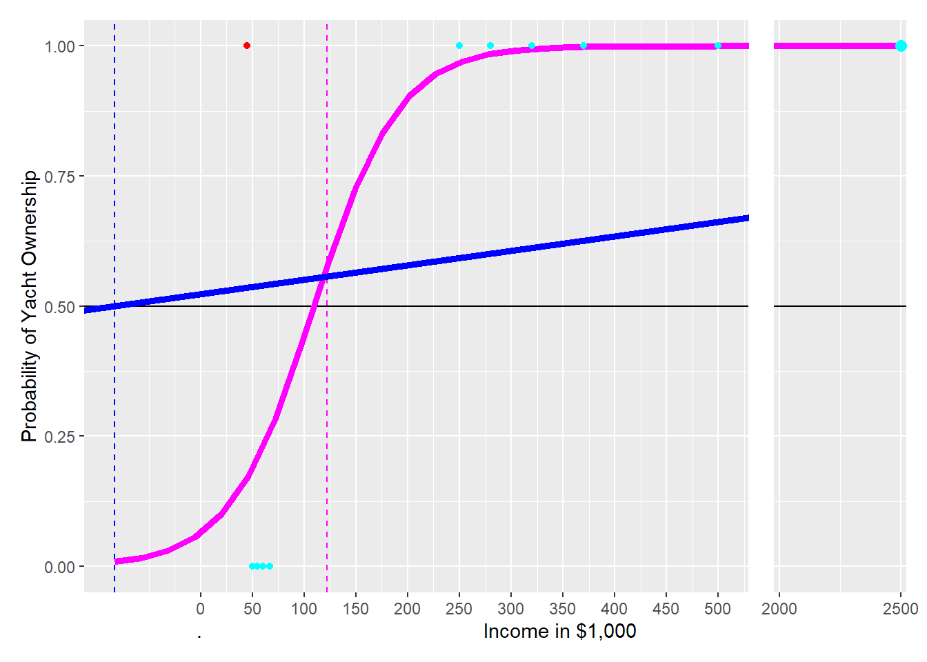
FIGURE 8.3: The Impact of an Oulier on Linear and Logistic Prediction Functions

To demonstrate this, let us add Nina’s observation to the training data and see what happens. Given Nina’s income ($2.5 million) and the fact that she owns a yacht \((Yacht=1)\), we get a new observation with an x-axis value of \(2{,}500\) far to the right and a y-value of \(1\) because Nina owns a yacht. Adding the observation for Nina to the training data changes both the logistic and the linear prediction function (see Figure 8.2):

• The new curve for the Logistic Regression (magenta) shifts a little to the right when adding the observation for Nina, but the shift is minimal. The decision boundary is now at 122 instead of 110. Therefore, the predictions from the Logistic Regression’s decision boundary have mostly stayed the same: Six of our friends with income greater than 122 are predicted correctly as yacht owners, including Nina’s prediction. Five of our friends with an income of less than 122 are predicted as not owning a yacht, which is correct for four of our friends but again not for Jack (red point).

• The new linear regression line — to better approximate the new data point — is much flatter than the original one (see the blue solid line). Consequently, the new decision boundary for the linear regression is now at an income of negative 83 (blue dashed line). This changes the predictions of the new linear prediction function dramatically compared to when the observation for Nina (the outlier) was not considered. All 11 observations are predicted as yacht owners because all 11 observations have an income greater than negative 83. This overly simplistic prediction leaves four observations with wrong predictions (compared to one with the Logistic Regression).

Linear regression is unsuitable for predicting categorical variables, because it is sensitive to outliers.

The question remaining is:

What is the advantage of the Logistic function compared to other Sigmoid (step) functions?

To approach this question, we must distinguish between odds and probabilities. You probably heard about odds already in connection with sports betting.

Probabilities vs. Odds

Both probabilities and odds measure the chance of a success (e.g., getting heads in a coin flip or rolling a six with a die).

A probability measures the ratio between the expected number of successes occurring in relation to the total number of possible events. For example, the probability of getting a head (success) in a coin flip is \(\frac{1}{2}=\frac{\#Successes}{\#Events}\), since we expect one head when we flip the coin twice. The probability of rolling a six with a die is \(\frac{1}{6}=\frac{\#Successes}{\#Events}\).

\[\begin{equation} P^{rob}_{yes}=\frac{\#Successes}{\#Successes+\#NoSuccesses} \end{equation}\]

In contrast, odds measure the ratio between the number of successes occurring in relation to the number of no-successes occurring. One could also say odds are the number of events with “something happening” in relation to the number of events with “something not happening”.

For example, the odds in a coin flip for heads are \(\frac{1}{1}=\frac{\#Successes}{\#NoSuccesses}\). The odds for rolling a six with a die are \(\frac{1}{5}=\frac{\#Successes}{\#NoSuccesses}\). We would say that the odds for heads are 1 to 1, often expressed as 1:1, and that the odds of rolling a six with a die are 1 to 5, often expressed as 1:5. You can calculate odds as:

\[\begin{equation} O^{dds}_{yes}=\frac{\#Successes}{\#NoSuccesses} \tag{8.3} \end{equation}\]

To derive how to convert probabilities to odds, we start with dividing numerator and denominator in Equation (8.3) by \((\#Successes+\#NoSuccesses)\):

\[\begin{equation} O^{dds}_{yes}=\frac{\frac{\#Successes}{\#Successes+\#NoSuccesses}} {\frac{\#NoSuccesses}{\#Successes+\#NoSuccesses}}=\frac{P^{rob}_{yes}}{P^{rob}_{no}} \tag{8.4} \end{equation}\]

You can see now that the main numerator in Equation (8.4) equals \(P^{rob}_{yes}\) and the main denominator equals \(P^{rob}_{no}\). Therefore, we can convert probabilities to odds as follows:

\[\begin{equation} O^{dds}=\frac{P^{rob}_{yes}}{P^{rob}_{no}}=\frac{P^{rob}_{yes}}{1-P^{rob}_{yes}} \quad\mbox{with: } P^{rob}_{no}=1-P^{rob}_{yes} \tag{8.5} \end{equation}\]

Now that you know what odds are, we can show you what makes the Logistic function so special. We start with the Logistic function from Equation (8.2):

\[P^{rob}_{yes,i}=\frac{1}{1+e^{-(\beta_1\cdot x_i+\beta_2)}} \] and take the reciprocal on both sides of the equation:

\[\frac{1}{P^{rob}_{yes,i}}=1+e^{-(\beta_1\cdot x_i+\beta_2)}\] Then we subtract 1 on both sides:

\[\frac{1}{P^{rob}_{yes,i}}-1=e^{-(\beta_1\cdot x_i+\beta_2)}\] When we consider that \(-1=-\frac{P^{rob}_{yes,i}}{P^{rob}_{yes,i}}\) and substitute \(-1\) accordingly, we get (after simplification):

\[\frac{1-P^{rob}_{yes,i}}{P^{rob}_{yes,i}}=e^{-(\beta_1\cdot x_i+\beta_2)}\]

Now we take again the reciprocal on both sides and get:

\[\frac{P^{rob}_{yes,i}}{1-P^{rob}_{yes,i}}=e^{\beta_1\cdot x_i+\beta_2}\] According to Equation (8.5) in the yellow box above, \(\frac{P^{rob}_{yes,i}}{1-P^{rob}_{yes,i}}=O^{dds}_{yes,i}\). If we substitute accordingly, we get:

\[\begin{equation} O^{dds}_{yes,i}=e^{\beta_1\cdot x_i+\beta_2}\tag{8.6} \end{equation}\] Equation (8.6) is the prediction equation for odds rather than probabilities as in Equation (8.2).

But there is another benefit from all the transformations. We can show this when we take the logarithm on both sides of Equation (8.7), resulting in Equation (8.7):

\[\begin{equation} \ln(O^{dds}_{yes/ln,i})=\beta_1 x_i+\beta_2 \tag{8.7} \end{equation}\]

The right-hand side of Equation (8.7) now shows a typical linear regression equation with one predictor variable. This allows us to interpret the coefficients, in our case \(\beta_1\), in a familiar way: We can say if \(x\) increases by one unit, the log odds on the left-hand side of Equation (8.7) increase by \(\beta_1\) units.

In addition, since the logarithmic change of a variable represents its percentage change, we can say that if \(x\) increases by one unit, then the odds increase by \(\beta_1\) percent. This means:

The coefficients in a Logistic Regression are directly interpretable.

One last comment before applying Logistic Regression to a real dataset: Unfortunately, we cannot use a formula, like in linear OLS, to calculate the optimal coefficients. Instead, we have to rely on an Optimizer to find the optimal \(\beta s\) by trial-and-error. However, this does not matter for practical purposes because the Optimizer is already built into the algorithm used by statistical software such as R.

8.4 🧭Analyzing Churn with Logistic Regression

Interactive Section

In this section, you will find content together with R code to execute, change, and rerun in RStudio.

The best way to read and to work with this section is to open it with RStudio. Then you can interactively work on R code exercises and R projects within a web browser. This way you can apply what you have learned so far and extend your knowledge. You can also choose to continue reading either in the book or online, but you will not benefit from the interactive learning experience.

To work with this section in RStudio in an interactive environment, follow these steps:

1. Ensure that both the learnR and the shiny package are installed. If not, install them from RStudio’s main menu (Tools -> Install Packages \(\dots\)).

2. Download the Rmd file for the interactive session and save it in your project folder. You will find the link for the download below.

3. Open the downloaded file in RStudio and click the Run Document button, located in the editing window’s top-middle area.

For detailed help for running the exercises including videos for Windows and Mac users we refer to: https://blog.lange-analytics.com/2024/01/interactsessions.html

Do not skip this interactive section because besides providing applications of already covered concepts, it will also extend what you have learned so far.

Below is the link to download the interactive section:

https://ai.lange-analytics.com/exc/?file=09-LogRegrExerc100.Rmd

Now that you have learned how Logistic Regression works, it is time to apply what you learned to a “real-world” problem.

In this interactive section, you are tasked to analyze churn behavior for customers of the Telco company. Telco is a fictional telecommunications company that offers various phone and Internet services. For your analysis, you will use the IBM Telco customer churn dataset (see IBM (2021)). In this dataset, the \(Churn\) column indicates if a customer departed within the last month \((Churn=Yes)\) or not \((Churn=No)\). Other columns contain various predictor variables for each of the 7,043 customers, such as \(Gender\) (\(Female\) or \(Male\)), \(SeniorCitizen\) (\(0\) for No or \(1\) for Yes), \(Tenure\) (months of membership), as well as \(MonthlyCharges\) (in U.S.-$).⁵⁵

The code block below has already been executed in the background for you. It loads the required libraries and the data, which then are stored in the R object DataChurn. Afterward, clean_names() changes the variable names to UpperCamel, and select() chooses the variables for the analysis. Finally, mutate() converts the outcome variable \(Churn\) to type factor, which is necessary because almost all tidymodels classification models require the outcome variable to be of type factor. The argument levels=c("Yes","No") ensures that “Yes” is treated as the positive class and “No” as the negative class. This is important when you later interpret metrics such as sensitivity and specificity:

library(rio); library(janitor); library(tidymodels)
DataChurn=import("https://ai.lange-analytics.com/data/TelcoData.csv") |>
          clean_names("upper_camel") |>
          select(Churn,Gender, SeniorCitizen, Tenure, MonthlyCharges) |>
          mutate(Churn=factor(Churn, levels=c("Yes", "No"))) 
head(DataChurn)

##   Churn Gender SeniorCitizen Tenure MonthlyCharges
## 1    No Female             0      1          29.85
## 2    No   Male             0     34          56.95
## 3   Yes   Male             0      2          53.85
## 4    No   Male             0     45          42.30
## 5   Yes Female             0      2          70.70
## 6   Yes Female             0      8          99.65

In the code block above, we used the mutate command to convert the outcome variable \(Churn\) into a factor variable. Why did we not use a recipe to accomplish the same goal? The reason is that conversion of outcome variables should always be done before splitting the data because manipulations of outcome variables are sometimes not executed on the test dataset when defined in a recipe. We already discussed this in Section 4.7.3. In addition, you can find more information about why recipes should not be used on outcome variables in Kuhn and Silge (2022), Section 8.4.

Now, it is your turn to split the data into training and testing data. You know how — right? Just substitute the ... (note that the data frame DataChurn has already been loaded in the background):

set.seed(789)
Split3070=...(..., prop=0.7, strata=...)

DataTrain=...(...)
DataTest=...(...)
head(DataTrain)

Before you create the recipe, the model design, and the workflow, you should take a look at the structure of the training dataset first. To show the structure of the R object DataTrain, we use the str() command on the data frame DataTrain in the code block below:

str(DataTrain)

## 'data.frame':    4929 obs. of  5 variables:
##  $ Churn         : Factor w/ 2 levels "Yes","No": 2 2 2 2 2 2 2 2 2 2 ...
##  $ Gender        : chr  "Female" "Male" "Male" "Female" ...
##  $ SeniorCitizen : int  0 0 0 0 0 0 0 0 0 0 ...
##  $ Tenure        : int  1 45 22 10 62 13 58 25 21 12 ...
##  $ MonthlyCharges: num  29.9 42.3 89.1 29.8 56.1 ...

You can see that \(Churn\) is a factor variable, which is what we want. \(SeniorCitizen\) is an integer dummy variable with \(1\) for senior citizens and \(0\) otherwise — no transformation needed. However, \(Gender\) should be a numerical dummy variable but is a character variable. Therefore, you need a step_dummy() in the recipe that transforms \(Gender\) into a dummy variable.

The other variables \(Tenure\) and \(MonthlyCharges\) are of type integer and double, respectively. Since this makes both variables numerical, no transformation is needed. Also, the Logistic Regression algorithm you will use later does not require normalization.

Consequently, the recipe has only one step — step_dummy() to convert \(Gender\) into a dummy variable. Please substitute the ... and then click Run Code to define RecipeChurn (note that the data frame DataTrain has already been loaded in the background):

RecipeChurn=recipe(...~., data=DataTrain) |> 
            step_...(Gender)
print(RecipeChurn)

To define the model design, you must set the algorithm’s name, the engine, and the mode. All of this is prepared for you in the code block below, and the code is already executed:

ModelDesignLogisticRegr=logistic_reg() |> 
                        set_engine("glm") |> 
                        set_mode("classification")

print(ModelDesignLogisticRegr)

## Logistic Regression Model Specification (classification)
## 
## Computational engine: glm

The printout above shows details about the model design. Now, you are ready to put it all together and fit the training data using the Optimizer to find the best \(\beta s\). Note that the recipe (RecipeChurn), the model design (ModelDesignLogisticRegr), and the training dataset (DataTrain) have already been loaded in the background:

WFModelChurn=workflow() |> 
             add_recipe(...) |> 
             add_model(...) |> 
             fit(...)
print(WFModelChurn)

After you execute the code above, the workflow model WFModelChurn can be used for predictions. We created WFModelChurn already in the background and again use the augment() command to predict the outcome variable based on the predictor variables from the testing dataset DataTest.

DataTestWithPred=augment(WFModelChurn, new_data=DataTest)
str(DataTestWithPred)

## tibble [2,114 × 8] (S3: tbl_df/tbl/data.frame)
##  $ .pred_class   : Factor w/ 2 levels "Yes","No": 2 2 2 2 2 1 2 2 2 1 ...
##  $ .pred_Yes     : num [1:2114] 0.1242 0.1027 0.1066 0.015 0.0801 ...
##  $ .pred_No      : num [1:2114] 0.876 0.897 0.893 0.985 0.92 ...
##  $ Churn         : Factor w/ 2 levels "Yes","No": 2 2 2 2 2 1 1 2 2 1 ...
##  $ Gender        : chr [1:2114] "Male" "Male" "Female" "Female" ...
##  $ SeniorCitizen : int [1:2114] 0 0 0 0 0 1 0 1 0 0 ...
##  $ Tenure        : int [1:2114] 34 16 69 52 71 1 1 71 27 5 ...
##  $ MonthlyCharges: num [1:2114] 57 18.9 113.2 20.6 106.7 ...

You can see in the printout that the data frame DataTestWithPred now includes columns for both the truth (\(Churn\)) and the estimate \((.pred\_class)\). Consequently, we can use DataTestWithPred to generate a confusion matrix:

conf_mat(DataTestWithPred, truth=Churn, estimate=.pred_class)

##           Truth
## Prediction  Yes   No
##        Yes  239  150
##        No   322 1403

Next, we create a new metrics command that we call FctMetricsSet. The FctMetricsSet() command takes the same arguments as the conf_mat() command and then outputs accuracy, sensitivity, and specificity:

FctMetricsSet=metric_set(accuracy, sensitivity, specificity)
FctMetricsSet(DataTestWithPred, truth=Churn, estimate=.pred_class)

## # A tibble: 3 × 3
##   .metric     .estimator .estimate
##   <chr>       <chr>          <dbl>
## 1 accuracy    binary         0.777
## 2 sensitivity binary         0.426
## 3 specificity binary         0.903

At a first glance, everything looks good. Accuracy is about \(78\%\), specificity is even \(90\%\). However, the result for sensitivity is not good. Only \(43\%\) of the customers who churned were correctly identified. Simply flipping a coin to determine if a customer churns or not would have given us a sensitivity of about \(50\%\)!

What went wrong?

Using the count() command in the code block below provides the answer:

count(DataTrain, Churn)

##   Churn    n
## 1   Yes 1308
## 2    No 3621

You can see the training dataset is not balanced. The number of observations in the training dataset for customers, who did not churn, is triple the number of observations for customers that did churn. This imbalanced dataset leads to a biased Optimizer with a tendency to predict \(Churn=No\).⁵⁶

The following section will introduce three algorithms that can help to fully or partially balance an imbalanced dataset. Afterward, in the interactive Section 8.6, you will apply your knowledge and repeat the Logistic Regression analysis performed in this section but with a more balanced dataset.

8.5 Balancing Data with Downsampling, Upsampling, and SMOTE

In the previous section, due to an imbalanced dataset, predictions were biased toward the over-represented \(Churn=No\) class, called the majority class. The majority class represents the most prevalent classification in a dataset. In contrast, the minority class represents the classification that occurs less often or rarely in a dataset (\(Churn=Yes\) in the Telco dataset).

A slightly imbalanced dataset usually does not cause any problems, but a dataset like the Telco dataset with 3,621 observations for the majority class and only 1,308 observations in the minority class (see Table 8.2 further below) can cause predictions biased toward the majority class.

The two most common approaches to work with imbalanced datasets are removing observations from the majority class (downsampling) and/or adding observations to the minority class (upsampling):

Downsampling:

This procedure randomly deletes observations from the majority class until the ratio of the observations from the majority and the minority class reaches the desired ratio (e.g., 1:1).

Upsampling:

In its simplest version, upsampling creates new observations for the minority class by copying randomly chosen observations from the minority class until the ratio of the observations from the majority and the minority class reaches the desired ratio (e.g., 1:1).

Often, a combination of downsampling and upsampling is performed.

Before working with up- and downsampling, we must decide whether to balance both the training and testing data or only the training data. The right decision is to balance the training data but not the testing data. This is because when the model is fully trained, the testing data are used to assess how the model will perform in the real world when facing new data in the production stage. Therefore, since the real world contains imbalanced data, the testing data should also contain imbalanced data neither treated with downsampling nor with upsampling.

In what follows, we will introduce one downsampling and two upsampling methods. These methods can be used in combination or individually. The themis package provides the related commands step_downsample(), step_upsample(), and step_smote(). These commands process, by default, only the training data but not the testing data.⁵⁷

Let us start with downsampling: In the code block below, we first load the themis package (Hvitfeldt (2023)) and then add step_downsample() to the recipe that we already used in Section 8.4 for the churn model.

library(themis)
set.seed(678)
RecipeChurn=recipe(Churn~., data=DataTrain) |> 
            step_dummy(Gender)|>
            step_downsample(Churn)

Later, we will add a similar recipe to a workflow, and the workflow will execute the recipe and thus balance the minority and majority classes.

At this point, we want to find out if the recipe successfully changes the composition of the training data. To test this, we must explicitly apply the updated recipe to the training data and store the results in a new data frame (DataTrainBal) for further analysis.

For this step, we can use the juice() command.⁵⁸ It extracts the training data from the recipe like a juicer squeezes lemon juice out of a lemon. Note, you have to add prep() after the recipe to ensure its execution before the data are extracted with juice().

DataTrainBal=RecipeChurn |> 
             prep() |> 
             juice()
count(DataTrainBal, Churn)

## # A tibble: 2 × 2
##   Churn     n
##   <fct> <int>
## 1 Yes    1308
## 2 No     1308

After using the count() command, you can see above that the dataset is now perfectly balanced. But when you compare the data from DataTrainBal with the original Telco training data (see Table 8.2), you also can see that we lost observations from the majority class because the majority class was reduced to 1,308 observations from 3,621 observations. Of course, losing so many records means losing a lot of information.

TABLE 8.2: Churn Count for Original Telco Training Dataset

Churn	n	Proportion
Yes	1308	0.2654
No	3621	0.7346

This brings us to upsampling. The idea behind upsampling is to randomly copy observations in the minority class until the number of observations in the minority class reaches the desired number of observations (the default is the same number as the majority class). The code block below is almost identical to the code blocks above, except that we use step_upsample() instead of step_downsample():

library(themis)
set.seed(678)
RecipeChurn=recipe(Churn~., data=DataTrain) |> 
            step_dummy(Gender)|>
            step_upsample(Churn) 

DataTrainBal=RecipeChurn |> 
             prep() |> 
             juice()
count(DataTrainBal, Churn)

## # A tibble: 2 × 2
##   Churn     n
##   <fct> <int>
## 1 Yes    3621
## 2 No     3621

As you can see when comparing the printout above with the contents of Table 8.2, the data set is balanced. However, we did not lose any observations because we increased the observations in the minority class.

In this context, it is important to point out that we do not gain any new information, although we now have more observations. This is because we copied existing observations to increase the minority class. The information contained in the training data did not increase!

Many data scientists believe that having multiple identical observations from upsampling in the minority class is not the best solution. Consequently, improved methods are needed to increase the number of observations in the minority class. One of these methods is SMOTE (Synthetic Minority Over-sampling Technique; see Chawla et al. (2002)). The idea behind SMOTE is to artificially generate new observations for the minority class, which are similar but not identical to existing observations. The SMOTE algorithm is implemented by the Themis package through step_smote() and works as follows:

1. Randomly choose an observation from the minority class.

2. Find the nearest neighbor to this observation using k-Nearest Neighbors (see Section 4 for details about the k-Nearest Neighbors algorithm).

3. Calculate a randomly weighted average for each predictor variable from the chosen observation from Step 1 and its nearest neighbor.

4. Use the calculated values for the predictor variables to create a new observation for the minority class.

Repeat Steps 1 – 4 until the number of observations in the minority class reaches the desired number of observations (the default is the same number as the majority class).

The code block below is identical to the code blocks above, except that we use step_smote():

library(themis)
set.seed(678)
RecipeChurn=recipe(Churn~., data=DataTrain) |> 
            step_dummy(Gender)|>
            step_smote(Churn) 

DataTrainBal=RecipeChurn |> 
             prep() |> 
             juice()
count(DataTrainBal, Churn)

## # A tibble: 2 × 2
##   Churn     n
##   <fct> <int>
## 1 Yes    3621
## 2 No     3621

The result in terms of observations in the minority and majority classes is the same as the one we got with step_upsample(). The improvement with SMOTE is that the observations in the minority class are now augmented with similar observations rather than identical copies of existing observations.

Later, in Section 8.6, you can experiment with the balancing methods introduced here, such as step_downsample(), step_upsample(), step_smote(), and you can combine them as you wish.

For the down- and upsampling commands step_downsample(), step_upsample(), and step_smote(), you can also set the desired ratio between the majority and minority class.

The Downsampling command uses the argument under_ratio= for the desired ratio. under_ratio is defined as:

\[\begin{eqnarray*} &&under\_ratio=\frac{N_{major}}{N_{minor}}\\ \mbox{with:}&& N_{major}:=\mbox{final number of observations for the majority class}\\ \mbox{and}&& N_{minor}:=\mbox{number of observations for the minority class} \end{eqnarray*}\]

For example, under_ratio=1 (the default) means that after downsampling is completed, the minority and the majority class have the same number of observations. under_ratio=1.2 means that downsampling will be stopped when the number of majority observations is 20% bigger than the number of minority observations.

For the two upsampling commands, step_upsample() and step_smote() the desired ratio is determined by the argument over_ratio=, which is defined as:

\[\begin{eqnarray*} &&over\_ratio=\frac{N_{minor}}{N_{major}}\\ \mbox{with:}&& N_{minor}:=\mbox{final number of observations for the minority class}\\ \mbox{and}&& N_{major}:=\mbox{number of observations for the majority class} \end{eqnarray*}\]

For example, over_ratio=1 (the default) means that after upsampling is completed, the minority and the majority class have the same number of observations. over_ratio=0.9 means that upsampling will be stopped when the number of minority observations reaches 90% of the number of observations of the majority class.

8.6 🧭Repeating the Churn Analysis with Balanced Data

Interactive Section

In this section, you will find content together with R code to execute, change, and rerun in RStudio.

The best way to read and to work with this section is to open it with RStudio. Then you can interactively work on R code exercises and R projects within a web browser. This way you can apply what you have learned so far and extend your knowledge. You can also choose to continue reading either in the book or online, but you will not benefit from the interactive learning experience.

To work with this section in RStudio in an interactive environment, follow these steps:

1. Ensure that both the learnR and the shiny package are installed. If not, install them from RStudio’s main menu (Tools -> Install Packages \(\dots\)).

2. Download the Rmd file for the interactive session and save it in your project folder. You will find the link for the download below.

3. Open the downloaded file in RStudio and click the Run Document button, located in the editing window’s top-middle area.

For detailed help for running the exercises including videos for Windows and Mac users we refer to: https://blog.lange-analytics.com/2024/01/interactsessions.html

Do not skip this interactive section because besides providing applications of already covered concepts, it will also extend what you have learned so far.

Below is the link to download the interactive section:

https://ai.lange-analytics.com/exc/?file=09-LogRegrExerc200.Rmd

When analyzing churn for the Telco company in Section 8.4 your results were biased toward predicting that customers do not churn \((Churn=No)\). This happened because the number of observations in the Telco dataset was biased toward customers who did not churn (the negative class).

As a reminder, due to the imbalanced dataset, specificity (prediction quality of the negative class) was \(90\%\), while sensitivity (prediction quality of the positive class) was only \(43\%\).

In this section, you will repeat the analysis from Section 8.4, but you will balance the training data before you perform the Logistic Regression analysis to improve the results. You will use the same training/testing data and the same commands (except for the recipe’s definition).

To give you an idea about how to modify the recipe, we present a first trial in the code block below. We use step_downsample(Churn, under_ratio=2) and step_smote(Churn, over_ratio=0.75):

set.seed(789)
RecipeChurn=recipe(Churn~., data=DataTrain) |> 
            step_dummy(Gender)|>
            step_downsample(Churn, under_ratio=2) |> 
            step_smote(Churn, over_ratio=0.75)

DataTrainBal=RecipeChurn |> 
             prep() |> 
             juice()
count(DataTrainBal, Churn)

## # A tibble: 2 × 2
##   Churn     n
##   <fct> <int>
## 1 Yes    1962
## 2 No     2616

How did we get the data frame DataTrainBal? First, step_downsample(Churn, under_ratio=2) randomly deletes observations from the majority class of the training data frame (DataTrain), until the number of observations in the majority class is reduced to double the size of the minority class (1,308 observations for \(Churn=Yes\) and 2,616 observations for \(Churn=No\)); initially the majority class was almost triple the size of the minority class. Afterward, step_smote(Churn, over_ratio=0.75) creates new observations for the minority class until the number of observations in the minority class reaches 75% of the number of observations of the majority class (1,962 observations for \(Churn=Yes\) and 2,616 observations for \(Churn=No\)).

Using this somehow more ballanced dataset, we get (based on the testing data), the following confusion matrix:

##           Truth
## Prediction  Yes   No
##        Yes  350  338
##        No   211 1215

The confusion matrix above implies a specificity of 78% but still only a sensitivity of 62%. This is an improvement compared to the analysis with the imbalanced dataset, but maybe you can improve the results even further.

You will use the code block further below to improve the results. It contains the recipe definition from above and is otherwise identical to the code we used for the imbalanced dataset before. The training dataset DataTrain and the testing dataset DataTest have already been loaded in the background.

When you execute the code block below unchanged, you will get the same results as in the example above. Try this first and then try to improve the results further by changing the under_ratio and the over_ratio values. You can also try to use only undersampling or only oversampling:

# Recipe
set.seed(789)
RecipeChurn=recipe(Churn~., data=DataTrain) |> 
            step_dummy(Gender)|>
            step_downsample(Churn, under_ratio=2) |> 
            step_smote(Churn, over_ratio=0.75)

# Model Design
ModelDesignLogisticRegr=logistic_reg() |> 
                          set_engine("glm")|> 
                          set_mode("classification")

# Building Fitting Workflow
WFModelChurn=workflow() |> 
  add_recipe(RecipeChurn) |> 
  add_model(ModelDesignLogisticRegr) |> 
  fit(DataTrain)

# Prediction with augment()
DataTestWithPred=augment(WFModelChurn, new_data=DataTest)

# Printing counts for traingdata after down- and upsampling
DataTrainBal=RecipeChurn |> 
             prep() |> 
             juice( )

print("Count for balanced training data:")
print(count(DataTrainBal,Churn))

# Creating Metrics Based on DataTest
ConfMatrix=conf_mat(DataTestWithPred,truth=Churn, estimate=.pred_class)

print("*confusion matrix*")
print(ConfMatrix)

FctMetricsSet=metric_set(accuracy, sensitivity, specificity)
FctMetricsSet(DataTestWithPred, truth=Churn, estimate=.pred_class)

8.7 When and When Not to Use Logistic Regression

• Logistic Regression is a straightforward algorithm and a good choice for predicting binary categorical variables. Because of its simplicity, Logistic Regression is also a fast algorithm in terms of required computing resources. Therefore, it can be used for large datasets.

• If it is crucial to interpret the impact of predictor variables in addition to predicting an outcome, Logistic Regression is a good choice. This is because, in contrast to many other classification algorithms, Logistic Regression allows the interpretation of its parameters.

• When logarithmic odds are estimated, Logistic Regression is algebraically similar to linear regression. This limits the non-linearity of the general prediction function. However, it also allows for a more straightforward interpretation of the predictor estimates.

• Logistic Regression might not be a well-suited method for complex or highly non-linear estimation problems. The reason is that the Logistic function, in its middle section, is almost linear. Consequently, for highly non-linear estimation problems, models such as Random Forest (see Chapter 10) or Neural Networks (see Chapter 9) are likely to be better alternatives.

• In general, a good strategy for classification problems is to start with Logistic Regression as a benchmark and then try to improve the results with other machine learning algorithms.

• Probit and Tobit algorithms (see Hanck et al. (2023) and McDonald and Moffitt (1980)) are closely related to Logistic Regression. Because of their similarity with Logistic Regression they have similar strengths and weaknesses.

8.8 Digital Resources

Below you will find a few digital resources related to this chapter such as:

• Videos
• Short articles
• Tutorials
• R scripts

These resources are recommended if you would like to review the chapter from a different angle or to go beyond what was covered in the chapter.

Here we show only a few of the digital resourses. At the end of the list you will find a link to additonal digital resources for this chapter that are maintained on the Internet.

You can find a complete list of digital resources for all book chapters on the companion website: https://ai.lange-analytics.com/digitalresources.html

Logistic Regression

A video from StatQuest by Josh Starmer. The video explains Logistic Regression in a fundamental and intuitive way.

Link: https://ai.lange-analytics.com/dr?a=393

Odds and Log(Odds), Clearly Explained!!!

A video from StatQuest by Josh Starmer. The video explains the difference between probabilities and odds. It also provides intuition for log-odds.

Link: https://ai.lange-analytics.com/dr?a=394

Undersampling, Oversampling, and SMOTE

An article by Joos Korstanje in Towards Data Science. The article introduces the problem of unbalanced data and explains undersampling, oversampling, as well as SMOTE. Although the examples are programmed in Python, they are easy to understand.

Link: https://ai.lange-analytics.com/dr?a=351

More Digital Resources

Only a subset of digital resources is listed in this section. The link below points to additional, concurrently updated resources for this chapter.

Link: https://ai.lange-analytics.com/dr/logregr.html

References

Aden-Buie, Garrick, Barret Schloerke, and JJ Allaire. 2022. Learnr: Interactive Tutorials for r. https://CRAN.R-project.org/package=learnr.

Chan, Chung-Hong, Geoffrey C. H. Chan, Thomas J. Leeper, and Jason Becker. 2021. Rio: A Swiss-Army Knife for Data File i/o.

Chang, Winston, Joe Cheng, JJ Allaire, Carson Sievert, Barret Schloerke, Yihui Xie, Jeff Allen, Jonathan McPherson, Alan Dipert, and Barbara Borges. 2022. Shiny: Web Application Framework for r. https://CRAN.R-project.org/package=shiny.

Chawla, Nitesh V., Kevin W. Bowyer, Lawrence O. Hall, and W. Philip Kegelmeyer. 2002. “SMOTE: Synthetic Minority over-Sampling Technique.” Journal of Artificial Intelligence Research 16. https://www.cs.cmu.edu/afs/cs/project/jair/pub/volume16/chawla02a-html/chawla2002.html.

Firke, Sam. 2023. Janitor: Simple Tools for Examining and Cleaning Dirty Data. https://CRAN.R-project.org/package=janitor.

Friedman, Jerome, Robert Tibshirani, and Trevor Hastie. 2010. “Regularization Paths for Generalized Linear Models via Coordinate Descent.” Journal of Statistical Software 33 (1): 1–22. https://doi.org/10.18637/jss.v033.i01.

Hanck, Christoph, Martin Arnoldand, Alexander Gerber, and Martin Schmelzer. 2023. Introduction to Econometrics with R. Online. https://www.econometrics-with-r.org/index.html.

Hvitfeldt, Emil. 2023. Themis: Extra Recipes Steps for Dealing with Unbalanced Data.

IBM. 2021. “Telco Customer Churn.” Online.

———. 2018. “Telco Customer Churn.” Online. https://www.kaggle.com/datasets/blastchar/telco-customer-churn/metadata.

Kuhn, Max, and Julia Silge. 2022. Tidy Modeling with r. A Framework for Modeling in the Tidyverse. O’Reilly, Sebastopol, CA. https://www.tmwr.org/.

Kuhn, Max, and Hadley Wickham. 2020. Tidymodels: A Collection of Packages for Modeling and Machine Learning Using Tidyverse Principles. https://www.tidymodels.org.

McDonald, John F., and Robert A. Moffitt. 1980. “The Uses of Tobit Analysis.” The Review of Economics and Statistics 62 (2): 318. https://doi.org/10.2307/1924766.

Tay, J. Kenneth, Balasubramanian Narasimhan, and Trevor Hastie. 2023. “Elastic Net Regularization Paths for All Generalized Linear Models.” Journal of Statistical Software 106 (1): 1–31. https://doi.org/10.18637/jss.v106.i01.

Verhulst, Pierre-François. 1845. “Recherches Mathématiques Sur La Loi D’accroissement De La Population” 18: 2013–15.

———. 2023d. “Sigmoid Function.” Wikipedia, the Free Encyclopedia. https://en.wikipedia.org/w/index.php?title=Sigmoid_function&oldid=1187110185.

Wooldridge, Jeffrey Marc. 2020. Introductory Econometrics: A Modern Approach. Seventh. Cengage Learning, Boston, MA. http://books.google.ch/books?id=64vt5TDBNLwC.

Zhu, Hao. 2021. kableExtra: Construct Complex Table with ’kable’ and Pipe Syntax. https://CRAN.R-project.org/package=kableExtra.

---

49. See Section 4.8 for the concepts of sensitivity and specificity.↩︎

50. See Wooldridge (2020), Section 7.5.↩︎

51. We neglect the problem of a probability being precisely \(0.5\).↩︎

52. A mitigation could be to define all probabilities greater than 100% as 100% and all negative probabilities as 0%. However, this would lead to a kinked prediction line and is also not a good solution for other reasons.↩︎

53. See Wikipedia contributors (2023d).↩︎

54. Confusingly the Logistic function is sometimes also called the Sigmoid function.↩︎

55. Note this dataset is from 2018 (Kaggle (2018)). If the data were collected today, most likely more \(Gender\) categories were considered.↩︎

56. The info box in Section 4.8 provides further details about how imbalanced datasets can cause prediction problems.↩︎

57. The skip= argument determines if a step_() command is applied to the testing data or if the testing data will be skipped. For most step_() commands, the default is skip=FALSE because usually, we want a step_() to be applied to the training and testing data. However, the default for step_downsample(), step_upsample(), and step_smote() is skip=TRUE to skip the testing data. You can change the default values for skip=, but it is not recommended.↩︎

58. In the book’s following chapters, we will not use juice(). Therefore, you do not need to memorize the juice() command.↩︎