Chapter 5 Linear Regression — Key Machine Learning Concepts

This is an Open Access web version of the book Practical Machine Learning with R published by Chapman and Hall/CRC. The content from this website or any part of it may not be copied or reproduced. All copyrights are reserved.

If you find an error, have an idea for improvement, or have a question, please visit the forum for the book. You find additional resources for the book on its companion website, and you can ask the experimental AI assistant about topics covered in the book.

If you enjoy reading the online version of Practical Machine Learning with R, please consider ordering a paper, PDF, or Kindle version to support the development of the book and help me maintain this free online version.

This chapter focuses on linear regression. Linear regression is a machine learning algorithm just like k-Nearest Neighbors (see Chapter 4), Random Forests (see Chapter 10.4), or Neural Networks (see Chapter 9). Assuming that most readers are familiar with the basics of linear regression, we will use linear regression as an example to introduce important machine learning concepts.

Therefore, even if you already have a good understanding of linear regression, you should read this chapter carefully as it introduces new machine learning concepts used in later chapters.

Section 5.4 introduces linear regression for a univariate (one predictor variable) approach. Based on a mockup dataset, two different approaches are used to optimize the regression parameters:

1. Ordinary Least Squares (OLS), which allows for calculating the regression parameters based on a formula.

2. Trial-and-Error algorithms which systematically try different regression parameters to improve the predictions.

   We will introduce Grid Search and an Optimizer based trial-and-error algorithm. These algorithms are widely used for more advanced machine learning models. This chapter will explain both algorithms, which allows us to treat them as black box concepts when working with other machine learning models in the following chapters.

In the interactive Section 5.5, you will work on an interactive project to extend the univariate model to a multivariate model using several predictor variables to estimate housing prices.

5.1 Learning Outcomes

This section outlines what you can expect to learn in this chapter. In addition, the corresponding section number is included for each learning outcome to help you to navigate the content, especially when you return to the chapter for review.

In this chapter, you will learn:

• The basic concepts of linear regression (see Section 5.3).

• How to calibrate parameters in a machine learning model to improve predictive quality (see Section 5.3).

• How to calculate optimal regression parameters using OLS (see Section 5.4.2).

• How to distinguish between unfitted and fitted models (see Section 5.4.2).

• How to use a trial-and-error algorithm called Grid Search in R to find optimal regression parameters (see Section 5.4.3.1).

• How to use an Optimizer trial-and-error algorithm in R to find optimal regression parameters (see Section 5.4.3.2).

• How to leverage the R tidymodels package to process data (recipes), to define a linear model (model design), to create a workflow, and to calibrate the workflow to the training data (see Section 5.4.2).

• How to transform categorical data such as the survival of a Titanic passenger (died/survived) or the waterfront location of a house (yes/no) into numerical dummy variables (see Section 5.5).

• How to distinguish between dummy encoding and one-hot encoding (see Section 5.5).

5.2 R Packages Required for the Chapter

This section lists the R packages that you need when you load and execute code in the interactive sections in RStudio. Please install the following packages using Tools -> Install Packages \(\dots\) from the RStudio menu bar (you can find more information about installing and loading packages in Section 3.4):

• The rio package (Chan et al. (2021)) to enable the loading of various data formats with one import() command. Files can be loaded from the user’s hard drive or the Internet.

• The janitor package (Firke (2023)) to rename variable names to UpperCamel and to substitute spaces and special characters in variable names.

• The tidymodels package (Kuhn and Wickham (2020)) to streamline data engineering and machine learning tasks.

• The kableExtra (Zhu (2021)) package to support the rendering of tables.

• The learnr package (Aden-Buie, Schloerke, and Allaire (2022)), which is needed together with the shiny package (Chang et al. (2022)) for the interactive exercises in this book.

• The shiny package (Chang et al. (2022)), which is needed together with the learnr package (Aden-Buie, Schloerke, and Allaire (2022)) for the interactive exercises in this book.

5.3 The Basic Idea Behind Linear Regression

The basic idea behind linear regression is to use a linear function with one (univariate) or more (multivariate) predictor variables \(x_j\) to predict a continuous outcome variable \(y\).

Equations (5.1) and (5.2) are examples of predicting the outcome \(y_{i}\) with one and two predictor variables, respectively. Because regression Equations (5.1) and (5.2) generate predictions for the true outcome variable \(y_i\), the variables on the left of the equations are marked with a hat (see \(\widehat{y}_i\)) to indicate that the left-hand-sides of Equations (5.1) and (5.2) are the results of predictions:³²

\[\begin{eqnarray} \widehat{y}_{i} & = & \beta_{1}x_{i}+\beta_{2} \tag{5.1}\\ \widehat{y}_{i} & = & \beta_{1}x_{1,i}+\beta_{2}x_{2,i}+\beta_{3} \tag{5.2} \end{eqnarray}\]

We know the numerical values for the predictor variables \(x_{j,i}\) for any given observation in the training and testing dataset. Consequently, we can plug in the numerical values for the predictors \(x_{j,i}\) into Equations (5.1) or (5.2) and calculate a prediction for the outcome \((\widehat{y}_{i})\).

However, this only works if and only if we know the values for the parameters (the \(\beta s\)). Finding optimal values for the parameters that result in the best prediction quality is the central objective for linear regression. It is similarly important for most machine learning algorithms.

In linear regression the term coefficients instead of parameters is often used for the \(\beta\) values. We choose the term parameters to be compatible with other machine learning algorithms in upcoming chapters.

We will introduce two methodologies for finding the optimal \(\beta s\):

Method 1:

Using Ordinary Least Squares (OLS) to calculate optimal values for the parameters \(\beta\). OLS is the default method for almost all statistical programs for linear regression, including R.

Method 2:

Using a systematic trial-and-error process to find optimal \(\beta\) parameters.

Both methods lead to approximately the same results. Therefore, it seems redundant to introduce a trial-and-error method when we can calculate the results precisely with OLS.

The reason for introducing trial-and-error approaches is that more complex machine learning algorithms do not allow us to calculate the optimal parameters, and we have to fall back onto trial-and-error approaches.

This chapter introduces two trial-and-error algorithms. This will allow us to treat these algorithms as a black box when we use them in the following chapters.

In the previous chapter, we used the confusion matrix to assess prediction quality. With linear regression, this is not possible because our outcome variable is continuous. Various metrics (see Section 6.4) are available to measure prediction quality for a continuous variable. For simplicity, throughout this chapter, we will only use the Mean Squared Error (\(MSE\)) to quantify prediction quality:

\[MSE=\frac{\sum_{i=1}^N (\widehat{y}_i-y_i)^2}{N}\]

Looking at the formula above, you can see why this metric is called Mean Squared Error. The term \((\widehat{y}_i-y_i)^2\) quantifies the (squared) error for each observation. So, summing over all squared errors and dividing by the number of observations gives us the Mean Squared Error.

5.4 Univariate Mockup: Study Time and Grades

To illustrate the OLS approach (see Section 5.4.2) and two different trial-and-error approaches (Grid Search in Section 5.4.3.1 and an Optimizer approach in Section 5.4.3.2), we use an extremly simplified mockup dataset consisting of only five observations. In the real-world five observations are surely not enough to perform a reliable data analysis! However, to keep it simple, we will ignore this fact for now.

The goal is to estimate the outcome of an exam based on students’ study time. The predicted outcome variable is \(\widehat {Grade}_i\) (similar to \(\widehat{y}_i\) in Equation (5.1)) and the only predictor variable is \(StudyTime_i\) (similar to \(x_i\) in Equation (5.1)).

Table 5.1 displays the five observations for both variables, \(Grade\) and \(StudyTime\), in Columns 2 and 3.

TABLE 5.1: Mockup Training Dataset

	\(y_i\)	\(x_i\)	\(\widehat{y}_i\)	\(\widehat{y}_i-y_i\)	\((\widehat{y}_i-y_i)^2\)
i	Grade	StudyTime	PredGrade	Error	ErrorSq
1	65	2	69	4	16
2	82	3	73	-9	81
3	93	7	89	-4	16
4	93	8	93	0	0
5	83	4	77	-6	36

5.4.1 Predictions and Errors

Before we analyze the relationship between \(StudyTime\) and \(Grade\) with linear regression, let us briefly introduce a few selected concepts related to predictions and the resulting errors:

Univariate Linear Regression assumes we can predict an outcome based on a linear relationship between the outcome variable and one predictor variable. This can be expressed in a prediction equation such as:

\[\begin{equation} \widehat{y}_i=\beta_{1}x_{i}+\beta_{2} \tag{5.3} \end{equation}\]

When numerical values for \(\beta_{1}\) and \(\beta_{2}\) are selected, we can use Equation (5.3) to predict the outcome \(\widehat{y}_i\) for each observation in the training or testing dataset (note, for simplicity, we do not consider a testing dataset here, but we will in Section 5.5).

The goal is to find optimal values \(\beta_{1,opt.}\) and \(\beta_{2,opt.}\) that maximize prediction quality.

Prediction quality can be measured through the Mean Square Error, which is defined as:

\[MSE=\frac{\sum_{i=1}^N (\widehat{y}_i-y_i)^2}{N}\]

The linear prediction equation for predicting the outcome \(Grade\) with the predictor \(StudyTime\) is:

\[\begin{equation} \widehat{Grade}_i=\beta_{1}StudyTime_i+\beta_{2} \tag{5.4} \end{equation}\]

Given a numerical pair of parameters (\(\beta_1\) and \(\beta_2\)), it is possible to predict a \(Grade\) for any value of the predictor variable \(StudyTime\). Let us arbitrarily choose \(\beta_1=4\), \(\beta_2=61\), and store the \(\beta' s\) in the R vector object VecBeta.

VecBeta=c(4, 61)
DataTable=DataMockup |> 
          mutate(PredGrade=VecBeta[1]*StudyTime+VecBeta[2])

The code block above shows how the predicted grade \((PredGrade)\) in Column 4 of Table 5.1) was calculated: In the mutate() command the values for \(\beta_1\) and \(\beta_2\) where extracted from VecBeta as VecBeta[1] (first element) and VecBeta[2] (second element) to calculate the variable \(PredGrade\).

Let us verify the predicted grade for the first observation in Table 5.1:

\[PredGrade_1=4\cdot 2 + 61= 69\]

The predicted grade for a student who studies for 2 hours is predicted to be 69 points. Similarly, you can predict the grades for all other observations in the training dataset (see Column 4 of Table 5.1). Try to verify at least one other observation’s \(PredGrade\)!

Figure 5.1 shows the \(StudyTime/Grade\) data from Table 5.1 plotted as blue points. The red line reflects the prediction equation for the arbitrarily chosen \(\beta_1=4\) and \(\beta_2=61\). Consequently, all predicted \(StudyTime/PredGrade\) combinations (black dots) are on the red line.

To measure the prediction error for each of the five observations (see Column 5 in Table 5.1), we have to calculate the difference between the prediction and the true value of the outcome variable:

\[Error=PredGrade-Grade\]

These errors are visualized in Figure 5.1 as the vertical difference between the blue points (true grades) and the black points (predicted grades).

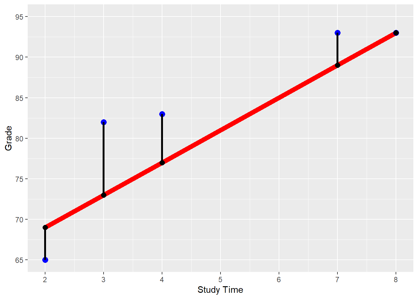
FIGURE 5.1: \(StudyTime\)/\(Grade\) Regression for \(\beta_1=4\) and \(\beta_2=61\)

In the code block below, the last two mutate() commands show how the values for the \(Error\) and the \(ErrorSq\) columns of Table 5.1 are calculated. You can also see that the \((MSE)\) is calculated from the mean of the observations squared error (\(ErrorSq\)):

DataMockup=
  import("https://ai.lange-analytics.com/data/DataStudyTimeMockup.rds")

VecBeta=c(4, 61)
DataTable=DataMockup |> 
          mutate(PredGrade=VecBeta[1]*StudyTime+VecBeta[2]) |> 
          mutate(Error=PredGrade-Grade) |> 
          mutate(ErrorSq=Error^2)
MSE=mean(DataTable$ErrorSq)
cat("The MSE for VecBeta[1]=4 and VecBeta[2]=61 is:", MSE )

## The MSE for VecBeta[1]=4 and VecBeta[2]=61 is: 29.8

We can also calculate the \(MSE\) algebraically:

\[\begin{eqnarray} MSE & = & \frac{1}{N} \sum_{i=1}^{N}(\widehat{y}_{i}-y_{i})^{2}\nonumber \\ & \Longleftrightarrow&\nonumber \\ MSE & = & \frac{1}{N} \sum_{i=1}^{N}(\underbrace{\overbrace{\beta_{1}x_{i}+\beta_2}^{\mbox{Prediction $i$}}-y_i}_{\mbox{Error $i$}})^2 \tag{5.5} \end{eqnarray}\]

At this point, you can already see that smaller prediction errors (i.e., absolute smaller values for \(\widehat y_i-y_i\)) lead to a smaller \(MSE\). Therefore, our error function is well suited as a metric to measure a model’s predictive quality and can be used to find optimal \(\beta\) parameters for the model later on.

Equation (5.5) allows us to calculate the \(MSE\) for any set of parameters \((\beta_{1},\beta_{2})\) because based on the training dataset, all values for the predictor variable (\(x_i\)) and the outcome variable (\(y_i\)) are known — leaving only \(\beta_1\) and \(\beta_2\) to be determined.

This can be shown for the mockup dataset, if we resolve the summation sign (\(\sum\)) in Equation (5.5) and also substitute \(y_i\) and \(x_{i}\) with the training data observations from Table 5.1 (remember, \(i\) is the index for the observation), we get Equation (5.6):

\[\begin{eqnarray} MSE & = & \frac{(\beta_1x_{1}+\beta_2-y_1)^2 +(\beta_1x_{2}+\beta_2-y_2)^2 + \cdots+ (\beta_1x_{5}+\beta_2-y_{5})^2}{5} \nonumber \\ & \Longleftrightarrow& \nonumber \\ MSE & = & \frac{1}{5}\left[ (\underbrace{\overbrace{\beta_1\cdot 2+\beta_2}^{\mbox{Prediction $1$}}-65}_{\mbox{Error $1$}})^2 +(\underbrace{\overbrace{\beta_1\cdot 3+\beta_2}^{\mbox{Prediction $2$}}-82}_{\mbox{Error $2$}})^2\right.\nonumber \\ & &\nonumber \\ && + (\underbrace{\overbrace{\beta_1\cdot 7+\beta_2}^{\mbox{Prediction $3$}}-93}_{\mbox{Error $3$}})^2 +(\underbrace{\overbrace{\beta_1\cdot 8+\beta_2}^{\mbox{Prediction $4$}}-93}_{\mbox{Error $4$}})^2\nonumber \\ & &\nonumber \\ && +\left. (\underbrace{\overbrace{\beta_1\cdot 4+\beta_2}^{\mbox{Prediction $5$}}-83}_{\mbox{Error $6$}})^2\right] \tag{5.6} \end{eqnarray}\]

Equation (5.6) shows that when the training data are given, the MSE is only based on the choice of the parameters — the \(\color{rubineredcl}\beta s.\)

Consequently, if you now substitute the previously arbitrary chosen values, \(\beta_1=4\) and \(\beta_2=61\), into Equation (5.6), you can take a calculator and find that \(MSE=29.8\). This is very cumbersome, but it might be a good exercise to fully understand the importance of Equation (5.6).

Although calculating the \(MSE\) is cumbersome for a human, writing a function in R to calculate the \(MSE\) based on a pair of \(\beta\)-values and a training dataset is relatively easy. Since such a function will be needed in the following sections, we created an R function (FctMSE()) to calculate the \(MSE\). This function can be imported in your R code with the import() command (see the code block further below).

For those who are interested in the underlying code and how to program a function in R, a link to a blog post is provided in the Digital Resource Section 5.7.

How to use the function FctMSE() is shown in the code block below:

library(rio)
FctMSE=import("https://ai.lange-analytics.com/source/FctMSE.rds")
VecBeta=c(4, 61)
MSE=FctMSE(VecBeta, data=DataMockup)
cat("The MSE for VecBeta[1]=4 and VecBeta[2]=61 is:", MSE)

## The MSE for VecBeta[1]=4 and VecBeta[2]=61 is: 29.8

First, the code for the function is downloaded with import() and stored in the R object FctMSE. Next, the values for \(\beta_1\) and \(\beta_2\) are stored in the R vector object VecBeta. Finally, the function calculates the \(MSE\) based on VecBeta and the mockup dataset DataMockup. The result is printed with the cat() command.

In the printout above, you can see that the \(MSE\) calculated by FctMSE() is the same as the one we calculated manually previously.

Takeaways from the MSE

The \(MSE\) for a univariate OLS regression with \(N\) observations can be calculated as:

\[MSE=\frac{1}{N} \sum_{i=1}^N \left ( \beta_1 x_i +\beta_2 - y_i \right )^2 \mbox{ with: $x_i$ and $y_i$ known from the training dataset.}\]

1. When the training data are given, only the choice of the \(\beta\) parameters determines the \(MSE\). Since both — the values for \(x_i\) and \(y_i\) — are part of the training dataset, the \(MSE\) depends only on the chosen values for the \(\beta\) parameters.

2. Since different values for \(\beta_1\) and \(\beta_2\) generate different \(MSE\)s, the goal is to find a pair of \(\beta\) parameters that leads to the smallest possible \(MSE\).

In the following Section 5.4.2, you will learn how to calculate the optimal values \(\beta_{1,opt.}\) and \(\beta_{2,opt.}\) for the mockup example using OLS. Afterward, in Section 5.4.3, we will introduce two algorithms that a computer can use for a systematic trial-and-error approach to find the optimal values \(\beta_{1,opt.}\) and \(\beta_{2,opt.}\).

5.4.2 Calculate Optimal Parameter Values Based on OLS

The most common method to find optimal values for the parameters (such as \(\beta_1\) and \(\beta_2\)) in linear regression is based on the Ordinary Least Squares (OLS) method. With OLS, a linear regression’s optimal \(\beta s\) can be determined using formulas (closed-form solution). Unfortunately, OLS works only for linear regression, and we have to rely on trial-and-error for most other machine learning models.

Below are the formulas for the optimal \(\beta s\) for a univariate regression based on a training dataset with \(N\) observations. As before, we abbreviate the outcome variable \(Grade\) with \(y\) and the only predictor variable \(StudyTime\) with \(x\):³³

\[\begin{eqnarray} \beta_{1,opt}&=& \frac {N \sum_{i=1}^N y_i x_i- \sum_{i=1}^N y_i \sum_{i=1}^N x_i} {N \sum_{i=1}^N x_i^2 - \left (\sum_{i=1}^N x_i \right )^2}\tag{5.7}\\ && \nonumber \\ \beta_{2,opt.}&=& \frac{ \sum_{i=1}^N y_i - \beta_1 \sum_{i=1}^N x_i} {N} \tag{5.8} \end{eqnarray}\]

You can see that the values for \(\beta_{opt,1}\) and \(\beta_{opt,2}\) are only based on data from the training dataset. The two equations might look pretty scary to some readers unfamiliar with summation notation. However, it is actually not that difficult to calculate the values for \(\beta_{opt,1}\) and \(\beta_{opt,2}\) if we use R.

Again, we use the mockup dataset (see Columns 2 and 3 of Table 5.2) to demonstrate how \(\beta_{opt,1}\) and \(\beta_{opt,2}\) can be calculated with R based on Equations (5.7) and (5.8).

TABLE 5.2: Mockup Training Dataset with Columns for \(y_ix_i\) and \(x_i^2\)

	\(y_i\)	\(x_i\)	\(y_i x_i\)	\(x_i^2\)
i	Grade	StudyTime	GradeXStudyTime	StudyTimeSquared
1	65	2	130	4
2	82	3	246	9
3	93	7	651	49
4	93	8	744	64
5	83	4	332	16

We start with the summation \(\sum_{i=1}^N x_i\). The term \(\sum_{i=1}^N x_i\) means that we sum up all \(x_i\) considering that \(i\) takes values starting from 1 and ending with \(N\) (\(N\) being 5 in our case). Because \(i\) is the row number in Table 5.1, \(\sum_{i=1}^N x_i\) stands for the sum of the \(x\) column in Table 5.1. The same applies to \(\sum_{i=1}^N y_i\).

With this knowledge, we can already use R to calculate \(\sum_{i=1}^N x_i\) and \(\sum_{i=1}^N y_i\):

SumOfX=sum(DataMockup$StudyTime)
SumOfY=sum(DataMockup$Grade)

At this point, we are not ready yet to calculate \(\beta_{1,opt}\) according to Equation (5.7) because the formula also requires calculating the sum from the product of the observations for \(y_i\) and \(x_i\) \((\sum_{i=1}^N y_i x_i)\) as well as the sum of the squares of the \(x_i\) values \((\sum_{i=1}^N x_i^2)\). However, we can use the mutate() command to add these variables to the data frame DataMockup and call the new resulting data frame DataTable:

DataTable=DataMockup |>
  mutate(GradeXStudyTime=Grade*StudyTime) |>
  mutate(StudyTimeSquared=StudyTime^2) 

Table 5.2 shows the resulting data frame DataTable.

Next, we calculate the sums of \(\sum_{i=1}^N y_i x_i\) and \(\sum_{i=1}^N x_i^2\) (see the code block below). When we plug in these sums together with the previously calculated sums \(\sum_{i=1}^N x_i\) and \(\sum_{i=1}^N y_i\) and the value for \(N\) (\(N=5\)) into Equation (5.7) we get \(\beta_{1,opt}\):

N=5
SumOfY=sum(DataTable$Grade)
SumOfX=sum(DataTable$StudyTime)
SumOfXY=sum(DataTable$GradeXStudyTime)
SumOfXSq=sum(DataTable$StudyTimeSquared)

Beta1opt=(N*SumOfXY-SumOfX*SumOfY)/(N*SumOfXSq-SumOfX^2)

cat("Based on the training dataset the optimal value for Beta1 =",   
    Beta1opt)

## Based on the training dataset the optimal value for Beta1 = 3.963

Afterward, we can plug in the value of \(\beta_{1,opt.}\) into Equation (5.8) together \(\sum_{i=1}^N y_i\) and \(\sum_{i=1}^N x_i\) to calculate \(\beta_{2,opt.}\):

Beta2opt= (SumOfY-Beta1opt*SumOfX)/N
cat("Based on the training dataset the optimal value for Beta2 =", 
    Beta2opt)

## Based on the training dataset the optimal value for Beta2 = 64.18

Hurrah, you just used OLS to find the optimal \(\beta\)-values for the mockup regression! The good news is that you do not need to memorize these formulas. They are already integrated into the statistical software R. To find the optimal parameters with R, you can use the command linear_reg() from the tidymodels package. The R code to create a linear regression workflow is mostly the same as the one explained in detail in the previous chapter (see Section 4.7.3):

library(tidymodels)
RecipeMockup=recipe(Grade~StudyTime, data=DataMockup)

ModelDesignLinRegr=linear_reg() |> 
                   set_engine("lm") |> 
                   set_mode("regression")

WFModelMockup=workflow() |> 
              add_recipe(RecipeMockup) |> 
              add_model(ModelDesignLinRegr) |> 
              fit(DataMockup)

1. Define and save the recipe that indicates which variable is the outcome and which is the predictor variable, together with the data argument. Note that we do not add any step_ commands for data pre-processing since we can use the mockup data as is.

2. Define the model design in three steps that determine:

   1. The name of the machine learning model (linear_reg()).

   2. The R package used for that model (lm).

   3. The mode used — which is either “classification” or “regression”.

3. Add the recipe and the model design to the workflow and fit the workflow to the data.

Note that we did not split the data into training and testing data. Consequently, we fit the workflow with the complete dataset DataMockup as the training dataset. This is only acceptable because our example is a mockup. In a real-world application splitting into training and testing data is an absolute must to avoid overfitting (more on overfitting in Chapter 6).

Fitting the workflow with fit(DataMockup) is when the parameters for the model design are calculated and saved within the workflow model WFModelMockup. A (workflow) model where the values for the parameters have been determined is called a fitted model. A fitted model can be used for prediction.

Fitted Model vs. Unfitted Model

An unfitted model is a prediction equation like Equation (5.4) in Section 5.4.1 or a model workflow that has not been fitted to the training data (i.e., if we omit fit(DataTrain) in the workflow code). An unfitted model already contains the rule of how predictions are built. Still, because the numerical values for the parameters (\(\beta s\)) are not determined — an unfitted model cannot be used to predict.

When we determine the optimal values for the parameters (\(\beta s\)) by minimizing the \(MSE\), we calibrate (fit) the model to the training data. The model becomes a fitted model.

A fitted model can be directly used for predictions because the numerical values for its parameters (\(\beta s\)) have been determined.

We can use the tidy() command to extract the parameters and other useful information. In general, the tidy() command extracts important information from various types of R objects and returns a data frame that can be saved for further processing. Here we output the data frame to the Console:

tidy(WFModelMockup)

## # A tibble: 2 × 5
##   term        estimate std.error statistic p.value
##   <chr>          <dbl>     <dbl>     <dbl>   <dbl>
## 1 (Intercept)    64.2       6.06     10.6  0.00180
## 2 StudyTime       3.96      1.14      3.48 0.0399

As you can see in the column titled estimate, the value for the parameter related to StudyTime \((\beta_{1,opt.})\) and the one related to the intercept of the prediction function (Intercept; \(\beta_{2,opt.}\)) are the same as the ones we calculate manually above. Using a real-world dataset, we will interpret the other columns from the tidy() output later in Section 5.5.

5.4.3 Trial-and-Error to find Optimal Parameters

The following sections will use two trial-and-error approaches to find the optimal \(\beta's\). Since we calculated \(\beta_{1,opt.}\) and \(\beta_{2,opt.}\) already in the previous section, we can use the results as a benchmark to see how well the trial-and-error approaches are performing.

\[\begin{eqnarray} MSE & = & \frac{1}{N} \sum_{i=1}^{N}(\widehat{y}_{i}-y_{i})^{2}\nonumber \\ & \Longleftrightarrow&\nonumber \\ MSE & = & \frac{1}{N} \sum_{i=1}^{N}(\underbrace{\overbrace{\beta_{1}x_{i}+\beta_2}^{\mbox{Prediction $i$}}-y_i}_{\mbox{Error $i$}})^2 \tag{5.9} \end{eqnarray}\]

Equation (5.9) provides again the formula to calculate the \(MSE\). For a given training dataset (all \(y_i\) and \(x_i\) are known), we can choose any pair \(\beta_1\) and \(\beta_2\), and use Equation (5.9) to calculate the related mean squared error (see Section 5.4 for details). However, rather than arbitrarily choosing values for \(\beta_1\) and \(\beta_2\), we will use more systematic approaches.

In Section 5.4.3.1, we will use Grid Search: First, we generate two vectors \(\beta_1\) and \(\beta_2\) containing various values, respectively. Then we will use R to generate all possible combinations for the \(\beta_1\) and \(\beta_2\) values. For each of the resulting pairs of \(\beta_1\) and \(\beta_2\), we will calculate the \(MSE\) and finally choose the pair with the lowest \(MSE\).

In Section 5.4.3.2, we will use an Optimizer to find optimal values for \(\beta_1\) and \(\beta_2\). An Optimizer is an iterative computer algorithm that can find optimal parameters to minimize or maximize a target function. In our case the \(MSE\) function (5.9) is the target function.

5.4.3.1 Finding Optimal Parameters Using Grid Search

This section uses the Grid Search algorithm to find the pair of \(\beta_{1,opt}\) and \(\beta_{2,opt}\) that minimizes the \(MSE\).

Let us start by deciding on a range for \(\beta_1\) and \(\beta_2\) and on how many values we would like to test for each \(\beta\). At the beginning of this section, we used \(\beta_1=4\) and \(\beta_2=61\), and the prediction results were not too bad. So, why not use a range around these values. We choose a range from 3 – 5 for \(\beta_1\) and a range from 50 – 70 for \(\beta_2\). For each, \(\beta_1\) and \(\beta_2\), we will generate about 20 values in the chosen range.

In the code block below, we generate a sequence of values for \(\beta_1\) ranging from \(3\) to \(5\) with an increment of \(0.1\). For \(\beta_2\), we choose values ranging from \(50\) to \(70\) with an increment of \(1\) resulting in 21 values for each, \(\beta_1\) and \(\beta_2\). These values are then assigned to the R vector objects VecBeta1Values and VecBeta2Values, respectively.

VecBeta1Values=seq(3, 5, 0.1)
VecBeta2Values=seq(50, 70, 1)

cat("First 5 values for beta1:",VecBeta1Values[1:5],"\n",
    "Last 5 values for beta1:",VecBeta1Values[17:21],"\n",
    "First 5 values for beta2:",VecBeta2Values[1:5],"\n",
    "Last 5 values for beta2:",VecBeta2Values[17:21])

## First 5 values for beta1: 3 3.1 3.2 3.3 3.4 
##  Last 5 values for beta1: 4.6 4.7 4.8 4.9 5 
##  First 5 values for beta2: 50 51 52 53 54 
##  Last 5 values for beta2: 66 67 68 69 70

As you can see above, we printed the first and the last five values for each vector object VecBeta1Values and VecBeta2Values.

Now we need all possible pairwise combinations of the values generated for \(\beta_1\) and \(\beta_2\). Because we generated 21 values for each \(\beta_1\) and \(\beta_2\), we will end up with a total of 441 \((21\cdot 21)\) combinations. Fortunately, we do not have to generate these combinations manually. The R command expand.grid() can generate the 441 combinations for us. We store the result in the data frame GridBetaPairs and print the first and last five pairs of \(\beta_1\) and \(\beta_2\):

GridBetaPairs=expand.grid(Beta1=VecBeta1Values, Beta2=VecBeta2Values)
print(GridBetaPairs[c(1,2,3,4,5,437,438,439,440,441),])

##     Beta1 Beta2
## 1     3.0    50
## 2     3.1    50
## 3     3.2    50
## 4     3.3    50
## 5     3.4    50
## 437   4.6    70
## 438   4.7    70
## 439   4.8    70
## 440   4.9    70
## 441   5.0    70

For each pair of \(\beta_1\) and \(\beta_2\) (each row in GridBetaPairs), we must calculate the \(MSE\) to find the pair with the smallest \(MSE\). Because this method is comprehensive but not computationally efficient, Grid Search is sometimes called a Brute Force approach.

Calculating the \(MSE\) for the \(\beta_1\) and \(\beta_2\) pairs is accomplished in the following code block with the apply() command. It applies a function (in this case, FctMSE(); see Section 5.4.1 for details about FctMSE()) to each of the rows of the data frame GridBetaPairs using the \(\beta_1\) and \(\beta_2\) pairs in each row together with the data frame DataMockup to calculate the related \(MSE s\).³⁴ These \(MSE\) values are then stored in the R vector object VecMSE and appended to the data frame GridBetaPairs as a new column using mutate().

FctMSE=import("https://ai.lange-analytics.com/source/FctMSE.rds")
VecMSE=apply(GridBetaPairs, FUN=FctMSE, data=DataMockup, MARGIN=1)

GridBetaPairs=mutate(GridBetaPairs, MSE=VecMSE)

head(GridBetaPairs)

##   Beta1 Beta2   MSE
## 1   3.0    50 379.2
## 2   3.1    50 360.4
## 3   3.2    50 342.2
## 4   3.3    50 324.5
## 5   3.4    50 307.4
## 6   3.5    50 290.9

The printout above shows the structure of the data frame GridBetaPairs after the \(MSE s\) for each \(\beta\)-pair have been appended.

We will not use the apply() command in the following chapters. Therefore, it is sufficient to understand that apply() calculates the \(MSE\) for each of the rows of GridBetaPairs.

The last step is to find the \(\beta\)-pair with the smallest \(MSE\). This is a little tricky: We first find the smallest \(MSE\) (using min(MSE)) and then use this smallest MSE to filter the data frame (MSE==min(MSE)). The result is the row with the smallest \(MSE\), which we save as BestModel and print afterward.

BestModel=filter(GridBetaPairs, MSE==min(MSE))

print(BestModel[1,])

##   Beta1 Beta2  MSE
## 1     4    64 20.8

As you can see in the printout, we get \(\beta_1=4\) and \(\beta_2=64\) with an \(MSE=20.8\). This deviates slightly from the calculated values from Section 5.4.2 where we obtained \(\beta_{opt,1}=3.96\) and \(\beta_{opt,2}=64.18\). This deviation should not come as a surprise. For the \(\beta_1\) range, we used an increment of 0.1, and for the \(\beta_2\) range, an increment of 1, leaving us with a coarse grid. Still, this coarse grid already had 441 rows for which the \(MSEs\) needed to be calculated.

We suggest that you try a finer grid. Copy the code block further below into an R script. The code includes all commands we used before but uses a finer grid by changing the increment for \(\beta_1\) from 0.1 to 0.01, creating 201 different \(\beta_1\) values ranging from 3 to 5 in steps of 0.01. The increment for \(\beta_2\) is changed from 1 to 0.1, creating 201 different \(\beta_2\) values ranging from 50 to 70 in steps of 0.1. Now the grid GridBetaPairs is more granular, but it also contains 40,401 rows \((201\cdot 201)\) with pairs of \(\beta s\). This means R has to calculate the \(MSE\) for 40,401 pairs of \(\beta s\). When you execute the new code, it will take a while. It took about 15 minutes on a computer with four cores and an Intel i5 processor — enjoy a coffee while waiting.

Spoiler alert: In the end, you will get parameters very close to the ones we calculated in Section 5.4.2 with OLS.³⁵

library(rio); library(tidyverse)
FctMSE=import("https://ai.lange-analytics.com/source/FctMSE.rds")
DataMockup=
  import("https://ai.lange-analytics.com/data/DataStudyTimeMockup.rds")

VecBeta1Values=seq(3, 5, 0.01) #creates 201 beta1 values
VecBeta2Values=seq(50, 70, 0.1)#creates 201 beta2 values

GridBetaPairs=expand.grid(Beta1=VecBeta1Values, Beta2=VecBeta2Values)
cat("GridBetaPairs has", nrow(GridBetaPairs), "rows.")

VecMSE=apply(GridBetaPairs, FUN=FctMSE,data=DataMockup,MARGIN=1)

GridBetaPairs=mutate(GridBetaPairs, MSE=VecMSE)

BestModel=filter(GridBetaPairs, MSE==min(MSE))
print(BestModel)

In summary, we can say that Grid Search finds optimal parameters if the solution is within the range used for the search and if the grid is fine enough. On the other hand, a more refined grid, unfortunately, increases computing time exponentially because the \(MSE\) for all combinations needs to be calculated.

We will use Grid Search in Chapter 6 when tuning hyper-parameters.

5.4.3.2 Finding Optimal Parameters Using an Optimizer

The Grid Search algorithm tries all possible pairwise \(\beta s\) combinations. However, as you saw, it can be very slow. This raises the question if it is really necessary to calculate the \(MSE\) for all pairs or if there is a more systematic approach.

Different types of Optimizers fill this void. In general, the process for an Optimizer to find an \(MSE\)-minimum can be described in four steps:

1. The Optimizer uses a first guess for the parameters to start the Optimizer process.

   For example, we use \(\beta_1=4\) and \(\beta_2=61\) as a first guess.

2. The Optimizer uses the error function to calculate the target \(MSE\)-value for the chosen parameters.

   We will use the function FctMSE() to calculate the \(MSE\) based on the training data and the \(\beta_1\) and \(\beta_2\) parameters.

3. The Optimizer changes the parameters slightly so that the new parameters result in a lower target value (a slightly lower \(MSE\)).

4. Repeat Steps 2 and 3 until the target value (\(MSE\)) approximately reaches a minimum.

The process described above leads to a local minimum. A local minimum guarantees that no \(\beta\)-combination with a lower \(MSE\) exists in the close vicinity of the minimum (similar \(\beta s\)). However, it is possible that the minimum found is not unique and other local minima exist. Some or all of these other local minima have a smaller \(MSE\).

In practice, the problem of a local minimum often is negligible. In some cases (including linear regression), we already know that only one minimum exists. In other cases, the predictive quality is already good, and it is not very relevant if we can further improve.

Most importantly, a very high approximation of the training data might lead to overfitting — approximating the training data well but predicting the testing data poorly (more in Chapter 6). Therefore, finding the lowest local minimum (global minimum) for the \(MSE\) for the training data might not be in our best interest. The old saying “Perfect is the enemy of the good”, applies.

The good message is that Optimizers are already integrated into almost all machine learning algorithms. They are executed automatically and can be treated as a black box.

In addition, R (like most statistical software packages) provides an Optimizer as a command that we can use to minimize error functions. The command is called optim(), and we will only use it in this section to find the optimal parameters for the \(\beta's\) for the mockup example.

In its default mode, the optim() command requires three arguments:

1. A vector with the initial guess of the values for the \(\beta s\). Here we use \(\beta_1=4\) and \(\beta_2=61\) (if you like, you can try to run the Optimizer with a different initial guess).

2. The name (without the parentheses) of the R function to be minimized. In this case, FctMSE.

3. The name of the data frame that contains the training data. In this case, data=DataMockup

library(tidymodels)
VecBetaFirstTrial=c(4, 61)
BestModel=optim(VecBetaFirstTrial, FctMSE, data=DataMockup)
cat("Optimal parameters values fo beta1 and beta2:", BestModel$par)

## Optimal parameters values fo beta1 and beta2: 3.963 64.18

cat("Minuimum MSE:", BestModel$value)

## Minuimum MSE: 20.79

The optim() command’s output is stored in the R object BestModel. We can extract the optimal parameters with BestModel$par and the minimal \(MSE\) with BestModel$value.

You can see that the optimal parameters \(\beta_{opt,1}\) and \(\beta_{opt,2}\) are similar to what we calculated in Section 5.4.2 with OLS. Remember, these parameters were found by trial-and-error and were not calculated using the OLS formula.

Optimizers as a Black Box

Most machine learning models have built-in Optimizers. We can treat them as black boxes:

An Optimizer is a black box. It finds the best parameters for an error function that only depends on the training data and a set of parameters.

This is all you need to know to understand the fitting process of machine learning models.

The fit(DatTrain) command from the tidymodels package pushes the training data to an internal Optimizer. Then the Optimizer finds the optimal parameter values for the \(\beta s\) and creates a fitted workflow that can be used for prediction.

5.5 🧭Project: Predict House Prices with Multivariate Regression

Interactive Section

In this section, you will find content together with R code to execute, change, and rerun in RStudio.

The best way to read and to work with this section is to open it with RStudio. Then you can interactively work on R code exercises and R projects within a web browser. This way you can apply what you have learned so far and extend your knowledge. You can also choose to continue reading either in the book or online, but you will not benefit from the interactive learning experience.

To work with this section in RStudio in an interactive environment, follow these steps:

1. Ensure that both the learnR and the shiny package are installed. If not, install them from RStudio’s main menu (Tools -> Install Packages \(\dots\)).

2. Download the Rmd file for the interactive session and save it in your project folder. You will find the link for the download below.

3. Open the downloaded file in RStudio and click the Run Document button, located in the editing window’s top-middle area.

For detailed help for running the exercises including videos for Windows and Mac users we refer to: https://blog.lange-analytics.com/2024/01/interactsessions.html

Do not skip this interactive section because besides providing applications of already covered concepts, it will also extend what you have learned so far.

Below is the link to download the interactive section:

https://ai.lange-analytics.com/exc/?file=05-LinRegrExerc100.Rmd

Now that you learned some details about OLS, Grid Search, and Optimizers based on a mockup dataset, it is time to work with a real-world scenario. In this section, you will work on a project to estimate housing prices with linear regression using the so-called King County House Sale dataset (Kaggle (2015)). This dataset contains house sale prices from May 2014 to May 2015 for King County in Washington State, including Seattle, WA.

As predictor variables, you will use:

\(Sqft\):

The living square footage of a house. This variable is called \(SqftLiving\) in the original dataset and therefore needs to be renamed to \(Sqft\).

\(Grade\):

Indicates the condition of a house ranging from 1 (worst) to 13 (best).

\(Waterfront\):

Indicates if a house is located at the waterfront. Being at a waterfront location is coded in the original dataset as \((Waterfront=yes)\) otherwise as \((Waterfront=no)\).

In the code block below, we import the complete King County dataset with all 21,613 observations using import(). Then we convert the variable names to UpperCamel style with clean_names("upper_camel") and select the variables \(Price\), \(Sqft\) (renamed from \(SqftLiving\)), \(Grade\), and \(Waterfront\).

It is unnecessary for a linear regression model to normalize the predictors as we did for the k-Nearest Neighbors model. The reason is that OLS adjusts the coefficients (\(\beta\) parameters) to changing dimensions. You find more information on why it is not necessary to normalize predictors for linear regression in the Digital Resource section for this chapter.

As in Chapter 4, we will split the data into training and testing data by randomly assigning observations to either the training or the testing data. As a reminder, only the training data are used to train the model (finding optimal parameters). The testing dataset is a holdout dataset exclusively used to assess the predictive quality after training has been completed.

library(tidyverse); library(rio); library(janitor); library(tidymodels)
DataHousing=
  import("https://ai.lange-analytics.com/data/HousingData.csv") |>
  clean_names("upper_camel") |>
  select(Price, Sqft=SqftLiving, Grade, Waterfront)
set.seed(777)
Split7030=initial_split(DataHousing, prop=0.7,  strata=Price, breaks=5)
DataTrain=training(Split7030)
DataTest=testing(Split7030)
head(DataTrain)

##    Price Sqft Grade Waterfront
## 1 221900 1180     7         no
## 2 180000  770     6         no
## 3 189000 1200     7         no
## 4 230000 1250     7         no
## 5 252700 1070     7         no
## 6 240000 1220     7         no

In the initial_split() command, the first argument (0.7) determines the proportion of observations randomly assigned to the training dataset (consequently, 30% are assigned to the testing dataset). The second argument (data=DataHousing) determines the data frame to be used as a source for the split. Like in Chapter 4, we choose one variable (strata=Price) that should be proportionally presented in the training and testing dataset. Since \(Price\) is a continuous variable rather than a categorical variable, we split the range of the housing prices into quintiles using breaks=5. This ensures observations from each quintile are proportionally represented in training and testing data. In the printout above, you can see the first six records of the training dataset.

The linear regression model is represented by the following equation:

\[\begin{equation} \widehat{Price}=\beta_1 Sqft+\beta_2 Grade+\beta_3 Waterfront\_yes +\beta_4 \tag{5.10} \end{equation}\]

OLS assumes that all predictor variables have an additive and independent impact on the outcome variable. The related \(\beta s\) scale the strength of these impacts.

Before using OLS to find the optimal numerical values for the \(\beta s\), we have to solve one more problem: The \(Waterfront\) variable in the data frame DataTrain is not numerical. Instead, it contains the values “yes” and “no”. To tackle this problem, we can turn \(Waterfront\) into a dummy variable using step_dummy() in the recipe. The command step_dummy() assigns a value of \(1\) when the value of the \(Waterfront\) variable is “yes” and a value of \(0\) when it is “no”. There is no definite rule about which value \(1\) or \(0\) is assigned to “yes” or “no”, but it is common practice to assign \(1\) to “yes” and \(0\) to “no”.

The recipe in the code block below determines the variables used for the analysis and converts \(Waterfront\) into a dummy variable. First, \(Price\) is defined as the outcome variable, and all other variables (\(Sqft\), \(Grade\), and \(Waterfront\)) are defined as predictor variables using the .-notation. Then step_dummy(Waterfront) converts the categorical variable \(Waterfront\) into the dummy variable \(Waterfront\_yes\).

library(tidymodels)
RecipeHouses=recipe(Price~., data=DataTrain) |> 
             step_dummy(Waterfront)

Note that step_dummy changes the variable name (the column name in the data frame) to indicate which category is set to “1”. Since waterfront “yes” is assigned to \(1\), the command step_dummy() renames \(Waterfront\) to \(Waterfront\_yes\). Consequently, if \(Waterfront\_yes=1\), a house is located at the waterfront.

Dummy Variables and One-Hot Encoding

A dummy variable is called a dummy because it fills in for the presence of a category. For example, the \(1\) of the dummy variable \(Waterfront\_yes\) indicates with a numerical value that a waterfront is present and with \(0\) that a waterfront is not present.

In the waterfront case, creating the dummy variable seems straightforward. However, in the case of red and white wines, one might create two dummy variables \(WineColor\_white\) and \(WineColor\_red\) with a value of \(WineColor\_white=1\) for white wines (\(0\) otherwise) and \(WineColor\_red\) for red wines (\(0\) otherwise). Creating a variable for each state of a categorical variable is called one-hot encoding.

One-hot encoding can be advantageous for some machine learning models (e.g., Random Forest) because it allows for a more straightforward interpretation of the variables. In OLS regressions one-hot encoding leads to a situation that makes it mathematically impossible to calculate the \(\beta s\) (dummy trap).

The dummy trap occurs when using one-hot encoding for OLS because one dummy variable is redundant. For example, in the case of white and red wines, when we know that \(WineColor\_white=1\), it follows that \(WineColor\_red=0\) (an observation (a wine) can be either white or red). This redundancy is also reflected in an algebraic property: If we know the values for \(WineColor\_white\), we can calculate the values for \(WineColor\_red\) (\(WineColor\_red=1- WineColor\_white\)). If we can calculate one predictor from one or more other predictor variables, these variables are perfectly correlated. The absence of perfect correlation is one of the conditions to be fulfilled for OLS regression.

Consequently, for OLS, if we have \(n\) categories, we will only consider \(n-1\) dummy variables. So, for example, in the case of the \(Waterfront\) categorical variable with two categories (“yes” and “no”), we will consider only one dummy variable \(Waterfront\_yes\) but not the other \(Waterfront\_no\) to avoid perfect correlation.

The multivariate model design for the housing analysis does not differ from the univariate model design in Section 5.4.2. From the package lm, we use the model linear_reg() with mode "Regression".

Please substitute the ... in the code block below and execute the code. If everything is correct, R prints information about the model design:

ModelDesignHouses=linear_reg() |> 
  set_engine("...") |> 
  set_mode("...")
print(ModelDesignHouses)

Next, you will use a pipe to add the recipe and the model design to a workflow and fit the workflow model to the training data.

Please substitute the ... in the code block below and execute the code. If everything is correct, R will print information about the fitted workflow model. The printout includes the optimal values for the \(\beta s\):

WFModelHouses=workflow() |>  
                add_recipe(...) |> 
                add_model(...) |> 
                fit(...)
print(WFModelHouses)

Another way to extract the optimal \(\beta\) values from the workflow object WFModelHouses is to use the tidy() command:

ResultsTidy=tidy(WFModelHouses)
print(ResultsTidy)

## # A tibble: 4 × 5
##   term           estimate std.error statistic   p.value
##   <chr>             <dbl>     <dbl>     <dbl>     <dbl>
## 1 (Intercept)    -570056.  15133.       -37.7 6.63e-297
## 2 Sqft               180.      3.25      55.2 0        
## 3 Grade            95214.   2548.        37.4 1.65e-292
## 4 Waterfront_yes  868338.  22200.        39.1 7.12e-319

The tidy() command returns the optimal \(\beta\) values and other information in a data frame. The resulting data frame is printed above. The estimate column contains values for the parameters for \(Sqft\) \((\beta_1)\), \(Grade\) \((\beta_2)\), \(Waterfront\_yes\) \((\beta_3)\), and the intercept \((\beta_4)\).

If we plug in the optimal \(\beta s\) in Equation (5.10), we get the prediction equation:

\[\begin{eqnarray} \widehat{Price}&=&180 \cdot Sqft+ 95214 \cdot Grade + \nonumber \\ && 868338 \cdot Waterfront\_yes + (-570056) \tag{5.11} \end{eqnarray}\]

If we know the values for the predictor variables, we can estimate the housing price. For example, if we want to predict the price of a house with 1,500 square feet (\(Sqft=1500\)), a building condition grade of \(9\) \((Grade=9)\), and the house is not located at the waterfront (\(Waterfront\_yes=0\)), we can plug in these values into the prediction Equation (5.11). As a result we get \(556{,}870\) as the predicted house price \((\widehat{Price}=556{,}870)\).

Try it out in the code block below. Substitute \(Sqft\), \(Grade\), and \(Waterfront\_yes\) with the corresponding values and execute the code to get the predicted price \((\widehat{Price})\).

180*Sqft+95214*Grade+868338*Waterfront_yes-570056

Equation (5.11) also helps to interpret the \(\beta s\). The \(\beta\) parameters indicate the predicted price change when the related predictor variable increases by one unit.

Suppose the living square footage increases by one unit (one extra square foot), then the estimated price of a house changes by about 180 units ($180) because the change of one unit is multiplied by 180 \((\beta_1=180)\). You can verify this when you return to the code block above and substitute \(Sqft\) with \(1501\) instead of \(1500\) (leave \(Grade=9\) and \(Waterfront\_yes=0\) unchanged). You will see that the estimated price will be $557,050 instead of $556,870, a change of $180.

The same interpretation is true for \(\beta_2\), the parameter for a building’s condition. If \(Grade\) increases by one unit (one grade), then the estimated price of that house increases by about $95,214 (confirm this in the code block above).

The interpretation of the parameter for the dummy variable \(Waterfront\_yes\) is a bit tricky. Technically, if the dummy variable \(Waterfront\_yes\) increases by one unit, the estimated housing price would increase by $868,338.

To better interpret this increase, we have to consider the limited range of a dummy variable: A dummy variable can only increase by one unit when it switches from \(0\) to \(1\). In the case of the \(Waterfront\_yes\) dummy, this means \(Waterfront\_yes=0\) increases by one unit to \(Waterfront\_yes=1\). In short, if we would hypothetically place a house that is not at the waterfront (\(Waterfront\_yes=0\)) to a location at the waterfront (\(Waterfront\_yes=1\)), the dummy variable \(Waterfront\_yes\) would increase by one unit — the estimated housing price would increase by $868,338. In other words, houses at the waterfront are expected to be $868,338 more expensive, on average.

Lastly, we need to check if the parameters are significant. The \(P\) values in the rightmost column from the tidy() command output above show the probabilities of the true parameters being zero (i.e., being irrelevant). Since the \(P\) values are all very close to zero, this probability is extremely low, meaning the parameters are significant.

The parameters’ interpretability and significance are strong points of linear regression. Unfortunately, most other machine learning models do not allow us to interpret their parameters directly. This is the reason why in the past these models were called black box models.

However, dramatic progress has been made in recent years that allows us to explain the predictions of machine learning models. We will introduce some important algorithms to better interpret the predictions of machine learning models in Chapter 11.

To assess the predictive quality of the fitted model based on the testing dataset (\(DataTest\)), we again use the augment() command. It predicts the housing price and appends the predictions as column .pred to the testing data. The resulting data frame is saved as DataTestWithPred:

DataTestWithPred=augment(WFModelHouses, DataTest)
head(DataTestWithPred)

## # A tibble: 6 × 6
##      .pred   .resid   Price  Sqft Grade Waterfront
##      <dbl>    <dbl>   <dbl> <int> <int> <chr>     
## 1 1450647. -220647. 1230000  5420    11 no        
## 2  404430. -146930.  257500  1715     7 no        
## 3  286802.    5048.  291850  1060     7 no        
## 4  416103. -186603.  229500  1780     7 no        
## 5  421491.  108509.  530000  1810     7 no        
## 6  816645. -166645.  650000  2950     9 no

You can see that the first observation has a predicted house price of $1,450,647. Since the testing dataset also includes the true value for the outcome variable \(Price\), you can calculate the prediction error (e.g., \(Error=1450647-1230000= 220647\)). The house was over-estimated by $ 220,647.

You might wonder why the data frame contains the character variable \(Waterfront\) and not the dummy variable \(Waterfront\_yes\). The answer is that predictions generated by augment() were appended to the original data frame DataTest, which contains the original categorical variable \(Waterfront\) with the values “yes” and “no”.

Since the data frame DataTestWithPred includes both the truth (\(Price\)) and the estimate (\(.pred\)), it allows using the metrics() command to evaluate the fitted model’s predictive quality for the testing data. Again, we only have to provide the truth=Price and estimate=.pred together with the date frame DataTestWithPred, and the metrics() command will calculate default metrics for the regression analysis:

metrics(DataTestWithPred,truth=Price, estimate=.pred)

## # A tibble: 3 × 3
##   .metric .estimator  .estimate
##   <chr>   <chr>           <dbl>
## 1 rmse    standard   244656.   
## 2 rsq     standard        0.549
## 3 mae     standard   163358.

As you can see above, the metrics() command calculates the root mean squared error (\(\sqrt{MSE}\); rmse), the \(r^2\) (rsq), and the mean absolute error (mae).

The rmse is closely related to the \(MSE\). A minimal \(MSE\) also implies a minimal root mean squared error. The importance of the \(MSE\) stems from the fact that it is used as a criterion to find the best parameters. However, the \(MSE\) and the rmse numerical values are not well suited for interpretation.

The \(r^2\) (rsq) expresses the proportion of the variance of the outcome variable (\(Price\)) explained by the prediction equation. In our case, the regression can explain 54% of the \(Price\) variance.

The most intuitive of the metrics calculated above is the mean absolute error (mae). The analysis performed here shows that based on the observations from the testing data, the model over/underpredicted the true housing price on average by $163,358.

5.6 When and When not to use Linear Regression

• An OLS regression can predict an underlying linear relationship between a continuous variable and one or more predictor variables. The resulting parameters are interpretable, and significance tests are possible if certain conditions (the Gauss-Markov conditions) are fulfilled (see Gujarati and Porter (2009) for more details).

• Linear regression is not a good choice if we face a classification problem like predicting if a wine is red or white. In Chapter 8 when Logistic Regression is covered, we will explain in detail why linear regression is ill-suited for classification.

• If the true relationship between the outcome and predictor variable(s) is non-linear, OLS regression is, in most cases, not a good tool to use. Although we can introduce some degree of non-linearity into a linear regression by transforming underlying data logarithmically before utilizing them as predictor and outcome variables, more complex non-linear relationships are unsuitable for OLS regression.

  

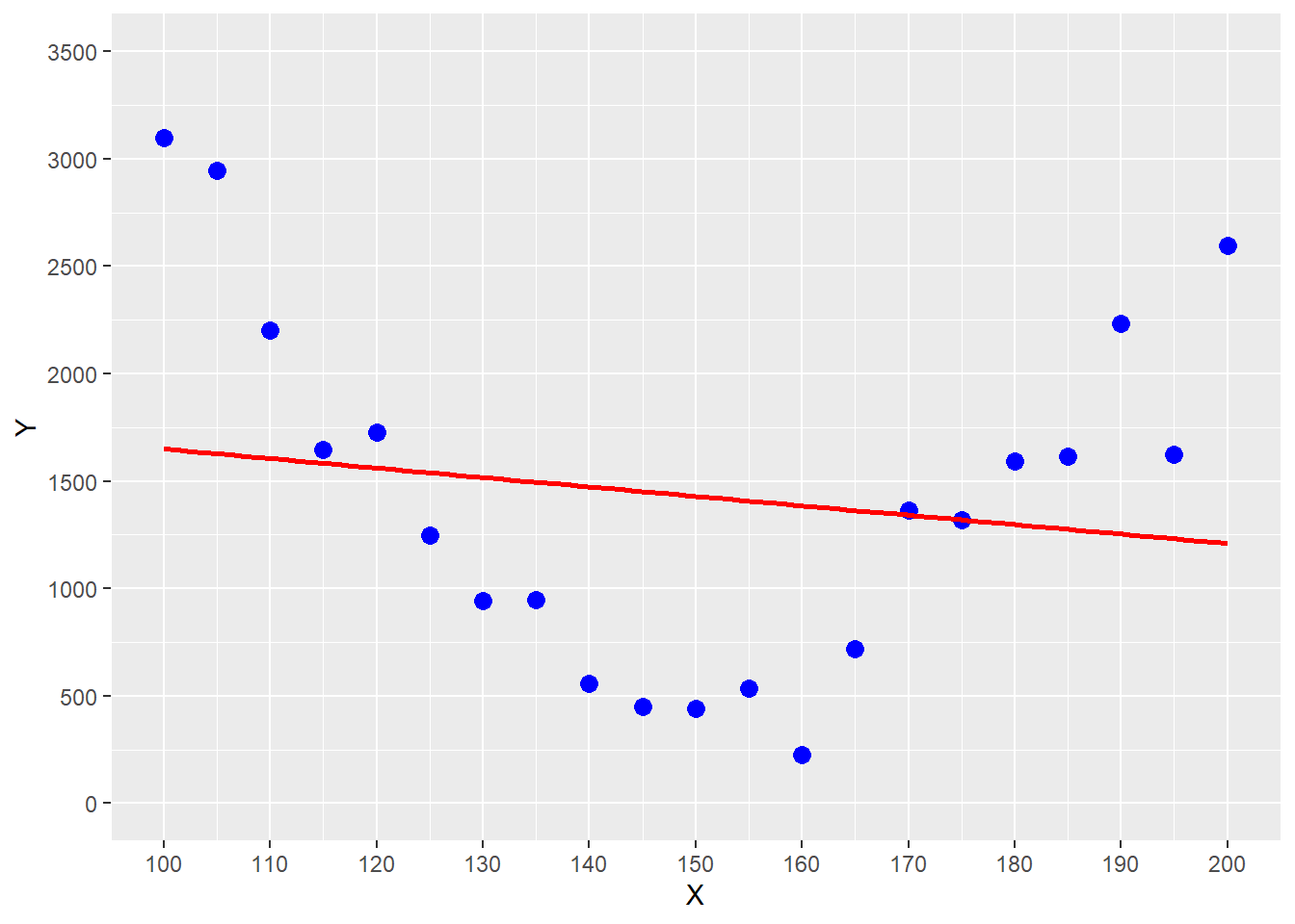
  FIGURE 5.2: Estimating a Parabolic Trend with OLS Regression

  You can see the problem in Figure 5.2, where the underlying relationship between the outcome variable \(Y\) and the predictor variable \(X\) follows a parabolic trend (see the blue data points). Using OLS on the data in Figure 5.2 would give us the red regression function. You can see that this regression function systematically underestimates for smaller predictor values (\(x \le 120\)), overestimates for values in the middle (\(120 < x \ge 165\)), and underestimates again for larger values (\(x \ge 180\)).

• It is possible to model basic interactions between predictor variables with OLS by transforming the data and thus indirectly introducing non-linearities (Chapter 7 provides an example).

  However, when using interaction terms, researchers must decide upfront which interactions to consider. In addition, interpreting the significance of the interaction terms can be problematic.

  If the goal is to consider more complex interactions and upfront assumptions about the type of interactions are difficult, other machine learning algorithms such as Neural Networks (see Chapter 9) or tree-based algorithms (see Chapter 10) are superior to OLS.

• In many cases it is a good idea to use linear regression as a benchmark and then evaluate if other more advanced machine learning models can deliver better predictive quality.

5.7 Digital Resources

Below you will find a few digital resources related to this chapter such as:

• Videos
• Short articles
• Tutorials
• R scripts

These resources are recommended if you would like to review the chapter from a different angle or to go beyond what was covered in the chapter.

Here we show only a few of the digital resourses. At the end of the list you will find a link to additonal digital resources for this chapter that are maintained on the Internet.

You can find a complete list of digital resources for all book chapters on the companion website: https://ai.lange-analytics.com/digitalresources.html

Linear Regression, Clearly Explained!!!

A video from StatQuest by Josh Starmer. The video explains the fundamentals of linear regression.

Link: https://ai.lange-analytics.com/dr?a=363

FctMSE() - An R Function to Calculate the Mean Squared Error

A blog post by Carsten Lange describes how to program an R function. It uses the R function FctMSE() which was used in the book Practical Machine Learning with R as an example. FctMSE() calculates the MSE for a dataset based on the provided parameter values for slope and intercept of a univariate prediction function.

Link: https://ai.lange-analytics.com/dr?a=362

Deriving the Formulas for Parameters in Univariate Linear Regression Using OLS

A blog post by Carsten Lange describes how optimal parameters for a univariate linear regression can be derived using the Ordinary Least Square method (OLS).

Link: https://ai.lange-analytics.com/dr?a=430

Why Predictors for Linear Regression Do Not Need Normalisation

This blog post by Carsten Lange describes why OLS linear regression data do not
need to be normalized. The article includes an example with R code showing how OLS
parameters (coefficients) adjust when dimensions change.

Link: https://ai.lange-analytics.com/dr?a=431

tidymodels Part 1: Running a Machine Learning Model in Three Easy Steps

This blog post by Carsten Lange shows that processing data, creating an OLS model design, and running the model requires only three steps in tidymodels. The blog post also shows that adjusting the code to use a different machine learning model requires only minimal modifications.

Link: https://ai.lange-analytics.com/dr?a=429

More Digital Resources

Only a subset of digital resources is listed in this section. The link below points to additional, concurrently updated resources for this chapter.

Link: https://ai.lange-analytics.com/dr/linregr.html

References

Aden-Buie, Garrick, Barret Schloerke, and JJ Allaire. 2022. Learnr: Interactive Tutorials for r. https://CRAN.R-project.org/package=learnr.

Chan, Chung-Hong, Geoffrey C. H. Chan, Thomas J. Leeper, and Jason Becker. 2021. Rio: A Swiss-Army Knife for Data File i/o.

Chang, Winston, Joe Cheng, JJ Allaire, Carson Sievert, Barret Schloerke, Yihui Xie, Jeff Allen, Jonathan McPherson, Alan Dipert, and Barbara Borges. 2022. Shiny: Web Application Framework for r. https://CRAN.R-project.org/package=shiny.

Firke, Sam. 2023. Janitor: Simple Tools for Examining and Cleaning Dirty Data. https://CRAN.R-project.org/package=janitor.

Gujarati, D. N., and D. C. Porter. 2009. Basic Econometrics. Economics Series. McGraw-Hill, New York, NY. https://books.google.com/books?id=6l1CPgAACAAJ.

Kaggle. 2015. “House Sales in King County, USA.” Online. https://www.kaggle.com/datasets/harlfoxem/housesalesprediction.

Kuhn, Max, and Hadley Wickham. 2020. Tidymodels: A Collection of Packages for Modeling and Machine Learning Using Tidyverse Principles. https://www.tidymodels.org.

Zhu, Hao. 2021. kableExtra: Construct Complex Table with ’kable’ and Pipe Syntax. https://CRAN.R-project.org/package=kableExtra.

---

32. Strictly speaking, the \(\beta s\) are also estimates and should be written as \(\widehat{\beta_j}\). For simplicity, in what follows, we omit the hats on model-parameters.↩︎

33. In the Digital Resource Section 5.7 you can find a link to a short blog article that shows how Equations (5.7) and (5.8) can be derived.↩︎

34. The argument Margin=1 ensures that the function FctMSE() is applied to the rows rather than the columns.↩︎

35. For those who like to push it a little further: Install the future.apply package and load it at the beginning of the code block with library(future.apply). Also, execute the command plan(multisession). Now when you rerun the code and change the apply() command to the future_apply() command (all arguments stay as they are), your code will be executed on different cores of your computer and should be much faster - assuming your computer has two or more cores.↩︎